
CONTENTS:
- A diagram showing self-similar derivative modulation for Fractal Taylor Series,
- A graph symbolizing scale-dependent damping behavior for Fractal Laplace Transform,
- A schema showing fractal orthogonality structure for Fractal Hilbert Space,
- A visual depicting micro-fluctuations around a black hole for Fractal Riemann Geometry,
- A self-similar density distribution curve for Fractal Probability Distributions,
- Fractal pole structures in the complex plane for Fractal Complex Analysis,
- A self-similar fluctuating exponential growth diagram for Fractal Functional Equations.
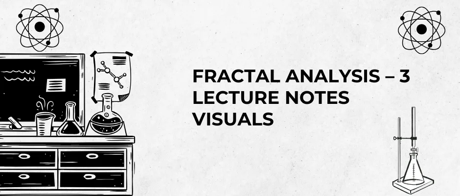
Fractal Taylor Series Visual
Fractal Taylor
In this diagram, the fractal extension of the classical Taylor expansion is visualized, where derivative terms become scale-dependent through self-similar modulations.
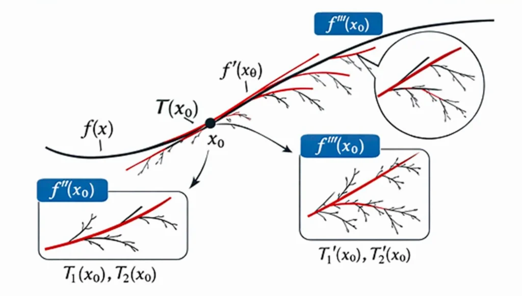
Fractal Laplace Transform Visual
This graph shows the fractal extension of the classical Laplace transform: damping behavior on the amplitude axis and self-similar resonances on the frequency axis.
The “Power Law” and “Exponential Decay” curves in the graph represent the two limits of scale-dependent damping; the magnifying glass on the right shows self-similar dampings in detail. This structure is used to model fractal damping behavior in the time domain in quantum systems.
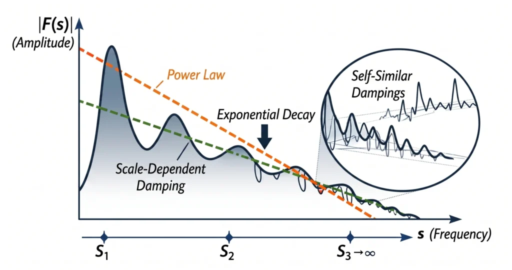
Fractal Hilbert Space Visual
This schema presents the representation of orthogonal vectors in an intertwined self-similar structure within fractal Hilbert space.
- The central section symbolizes the orthogonality of independent vectors: v₁ ⊥ v₂ and v₃ ⊥ v₁.
- In the four surrounding sub-diagrams, repeating fractal orthogonal structures at smaller scales are shown: sub-vector pairs such as v₁₁, v₁₂, v₂₁, v₂₂ each form right angles in their own planes.
- Dotted lines show the connection of these subspaces to the main central space and the multi-scale continuity of fractal orthogonality.
This structure is used to model the scale-dependent orthogonality of wave functions in fractal functional analysis.
Fractal Riemann Geometry Visual
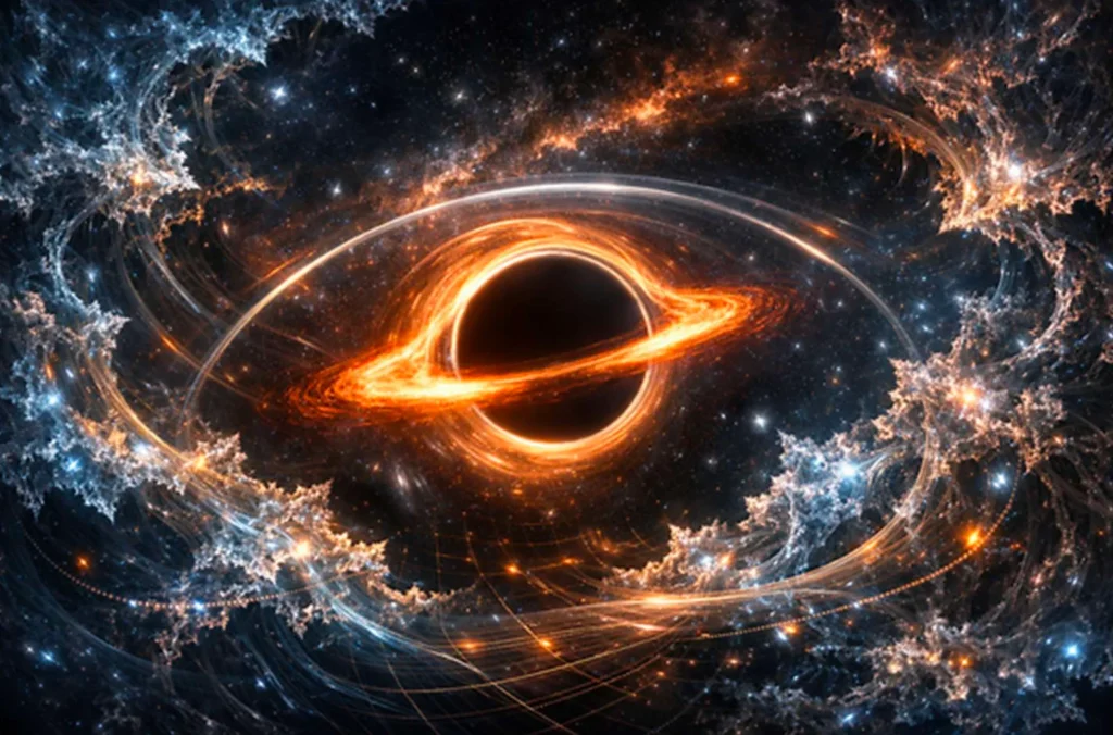
This digital illustration depicts fractal fluctuations of space-time around a black hole.
The central black hole is surrounded by a bright orange-yellow accretion disk rotating around it; light bends around the event horizon, creating a gravitational lensing effect. The blue, purple, and white-toned fractal space-time structures seen around it represent micro-scale curvature fluctuations. These fluctuations visualize the expanded version of the classical Riemann metric with fractal modulation:
𝑑𝑠2 = 𝑔μ𝛖 (𝑥) ⋅ 𝜙(𝑥) 𝑑𝑥μ𝑑𝑥𝛖
The warped grid surface at the bottom shows how space-time is bent by the gravitational pull of the black hole. This structure is the visual counterpart to the concepts of fractal curvature tensor and fractal geodesics.
Fractal Probability Distributions Visual
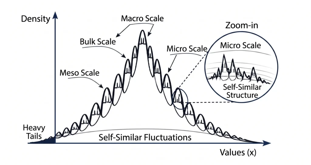
This graph shows the fractal extension of the classical probability density curve:
- The vertical axis is labeled “Density”, and the horizontal axis is labeled “Values (x)”.
- The curve begins with a large peak at the center (Macro Scale) and continues as smaller, self-similar peaks (Medium Scale and Micro Scale) as it moves to the right.
- The magnifying glass on the right emphasizes the “Self-Similar Structure”; here, fluctuations in the tail of the distribution show the micro-level effect of fractal modulation.
- The “Heavy Tails” and “Self-Similar Fluctuations” labels at the bottom highlight the difference between fractal distributions and the classical normal distribution.
This structure is used to analyze multi-scale probability resonances in fields such as quantum chaos and financial modeling.
Fractal Complex Analysis Visual
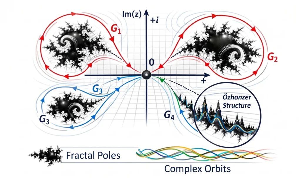
This illustration shows the self-similar resonance of fractal pole structures and contour integrals in the complex plane.
The complex plane, defined by Re(z) and Im(z) axes, is at the center; around it are fractal pole sets (G₁, G₂, G₃, G₄) surrounded by red and blue contour lines.
- Red contours represent resonance rings around the fractal Cauchy integral.
- Blue contours show regions of fractal residue calculation.
- The “Fractal Poles” and “Complex Trajectories” labels at the bottom emphasize the self-similar behavior of wave-particle interactions in the complex plane.
This structure is used in quantum field theory to model the resolution of wave functions through fractal resonance.
Fractal Functional Equations Visual
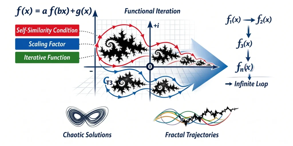
This diagram visualizes the fractal extension of the classical functional equation:
𝑓(𝑥 + 1) = 𝑎 ⋅ 𝑓(𝑥) ⋅ Φ(𝑥)
The basic equation is on the left; below it are three main concept boxes: Self-Similarity Condition, Scaling Factor, and Iterative Function. The large arrow pointing right in the middle represents the Functional Iteration process—the fractal fluctuating structure formed by the function converting its own output into input at each step. On the right, the iterative chain leading to an infinite loop is shown: 𝑓1(𝑥) → 𝑓2(𝑥) → 𝑓3(𝑥) → ⋯ → 𝑓𝑛(𝑥).
Two important results are highlighted at the bottom:
- Chaotic Solutions: Self-similar functional iterations producing chaotic attractors.
- Fractal Trajectories: The outputs of the function branching in a fractal manner to form trajectories in space.
This structure forms the mathematical foundation of self-similar dynamics in quantum chaos, financial systems, and astrophysical models.
Fractal Topology Visual
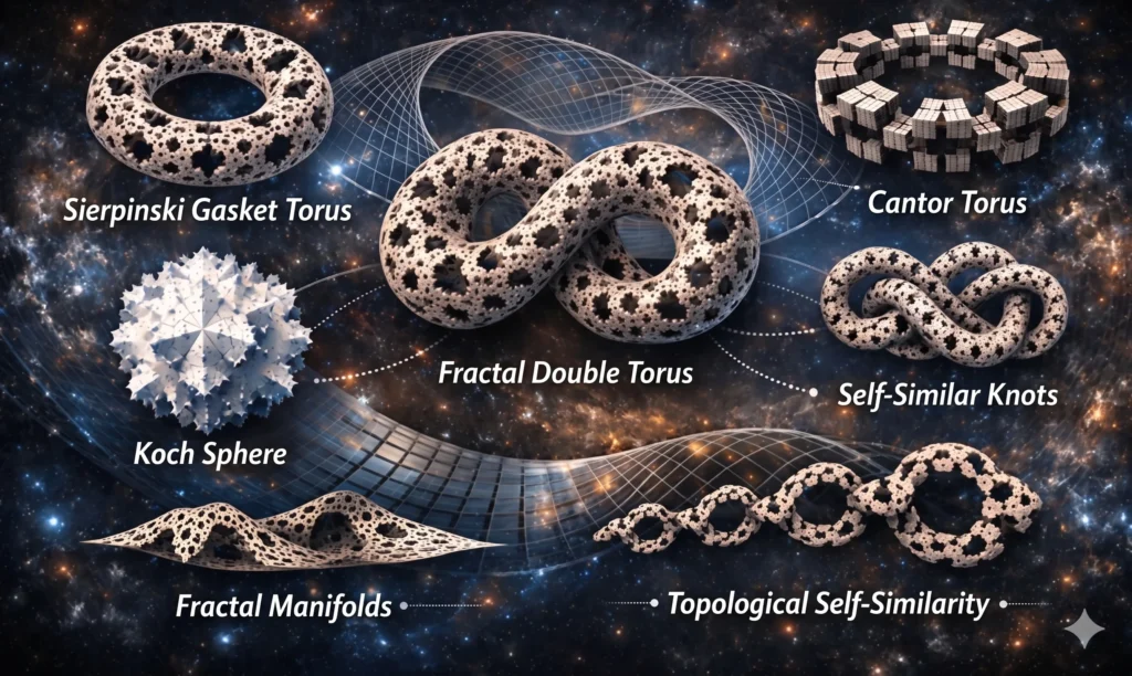
This illustration depicts the fractal extension of classical topology at the levels of space, continuity, and homotopy.
On the left are the Sierpinski Ring and Koch Sphere—symbolizing the self-similar transformation of open and closed sets into each other. The Fractal Double Torus in the center shows a structure where two intertwined tori are connected to each other by fractal surfaces; this is the geometric counterpart of fractal homotopy classes. On the right, Cantor Tori and Self-Similar Knots represent disconnected yet topologically connected fractal manifolds.
The cosmic scene in the background emphasizes the concept of continuity and connection of fractal topology at universal scales. At the bottom, Fractal Manifolds and Topological Self-Similarity labels summarize the transformation of multi-scale spaces into each other.
Fractal Differential Geometry Visual
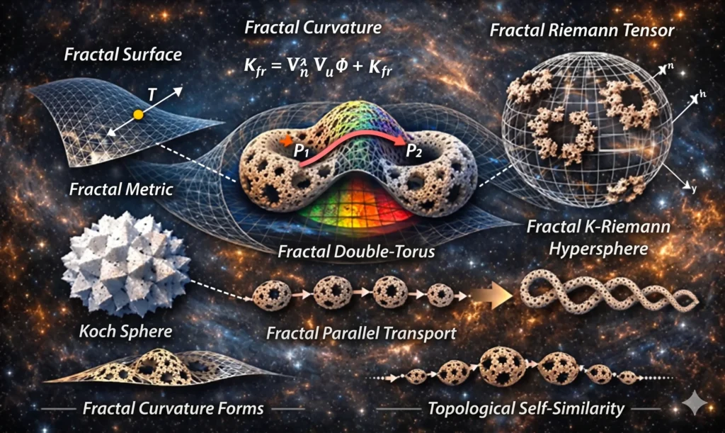
This illustration depicts space-time fractal curvature fluctuations and the fundamental components of fractal Riemann geometry.
On the left, a point 𝑃 on a Fractal Surface and a tangent vector 𝑇 are seen; this represents the formula for the fractal metric:
𝑑𝑠2 = 𝑔μ𝛖 (𝑥) ⋅ 𝜙(𝑥) 𝑑𝑥μ𝑑𝑥𝛖
The 3D surface in the center is shown as a Fractal Geodesic (red curve) along with colored contour lines; this curve expresses the fractal parallel transport process and curvature form.
On the right is the Fractal K-Riemann Hypersphere—a sphere with fractal patterns on its surface, along with coordinate axes 𝑥k and 𝑥𝑛. This structure symbolizes the fractal Riemann tensor:
𝑅𝑓r (𝑥) = 𝑅μ𝛖σλ (𝑥) ⋅ Φ(𝑥)
The Fractal Curvature Forms and Fractal Parallel Transport labels at the bottom form the visual counterpart of multi-scale geodesics and curvature resonances.
Fractal Statistical Processes Visual
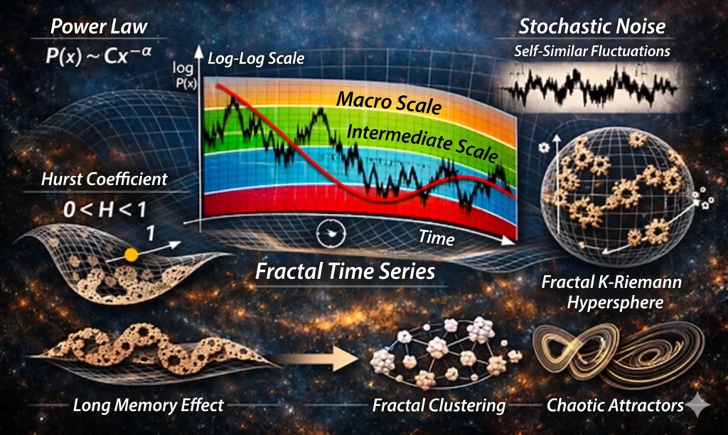
This infographic shows the fundamental components of multi-scale fractal stochastic processes:
- At the top left, the Power Law 𝑃(𝑥) ∼ 𝐶𝑥-𝑎 and Log-Log Scale graph emphasize the heavy-tailed nature of fractal distributions.
- The Fractional Noise section at the top right presents the visual counterpart of scale-dependent variance with its self-similar fluctuations.
- The Fractal Time Series in the center is drawn as a multi-layered signal fluctuating at macro, medium, and micro scales; this represents the long-memory effect.
- The Hurst Exponent (0 < H < 1), Fractal Clustering, and Chaotic Trajectories sections at the bottom show the self-similar structure of stochastic processes and their relationship with chaotic attractors.
This structure is used to resolve fractal statistical resonances in financial modeling, biological process analysis, and quantum chaos studies.
Fractal Entropy and Information Measures Visual
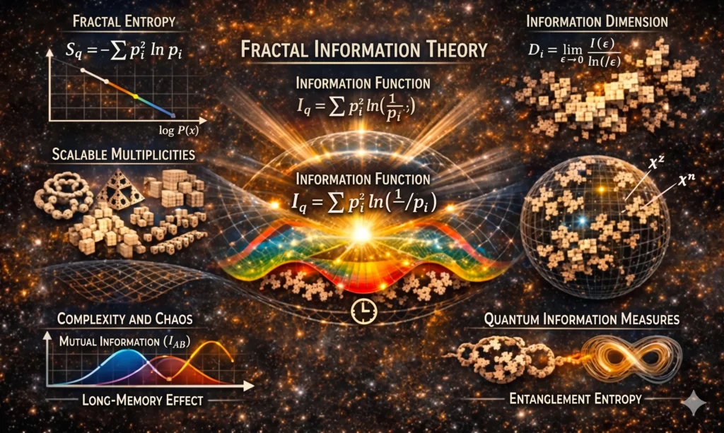
This infographic visualizes the fractal extension of information theory and scale-dependent uncertainty measurement in quantum systems.
- The Fractal Entropy section is at the top left; under the formula 𝑆q = −∑𝑝𝑖q ln𝑝𝑖 , scalar multiplicities—Sierpinski triangle, Cantor set, and fractal cube sets—are shown.
- In the Information Dimension part at the top right, fractal information sets are depicted as glowing square grids with the formula 𝐷 = lim𝜀→0 [𝐼(𝜀)/ln (1/𝜀)].
- Under the title Fractal Information Theory in the center is the information function 𝐼q = ∑𝑝𝑖q ln (1/𝑝𝑖); a spherical network emitting beams of light around it symbolizes the fractal resonance of information density.
- The Complexity and Chaos section in the bottom left corner shows the mutual information graph (curves A and B) between two systems.
- In the Quantum Information Criteria part at the bottom right, intertwined fractal spheres represent the concept of entanglement entropy.
This structure is used in quantum information theory to model the multi-scale analysis of uncertainty and information density with fractal entropy.
Fractal Homotopy Visual
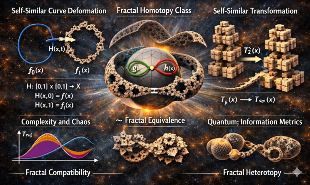
This illustration depicts the fractal extension of the classical homotopy concept—namely, the transformation of functions into each other through self-similar deformations.
On the left is Self-Similar Curve Deformation: a simple closed curve 𝑓0(𝑥) transforms into curve 𝑓1(𝑥) modulated with fractal branchings. The arrow in between represents the fractal homotopy function 𝐻(𝑥, 𝑡). The Fractal Homotopy Class in the center shows the fractal equivalence (≃) of two functions 𝑔(𝑥) and ℎ(𝑥) on a fractal-patterned Möbius strip. On the right, the Self-Similar Transformation section symbolizes the transformation of fractal cube towers extending iteratively to infinity (𝑇𝑛(𝑥) → 𝑇∞(𝑥)).
The Fractal Compatibility and Fractal Heterotopy labels at the bottom show the resonant transition of interconnected fractal spaces. This structure is used in fractal topology to model homotopy classes of self-similar deformations and quantum resonant transformations.
Fractal Homology Visual
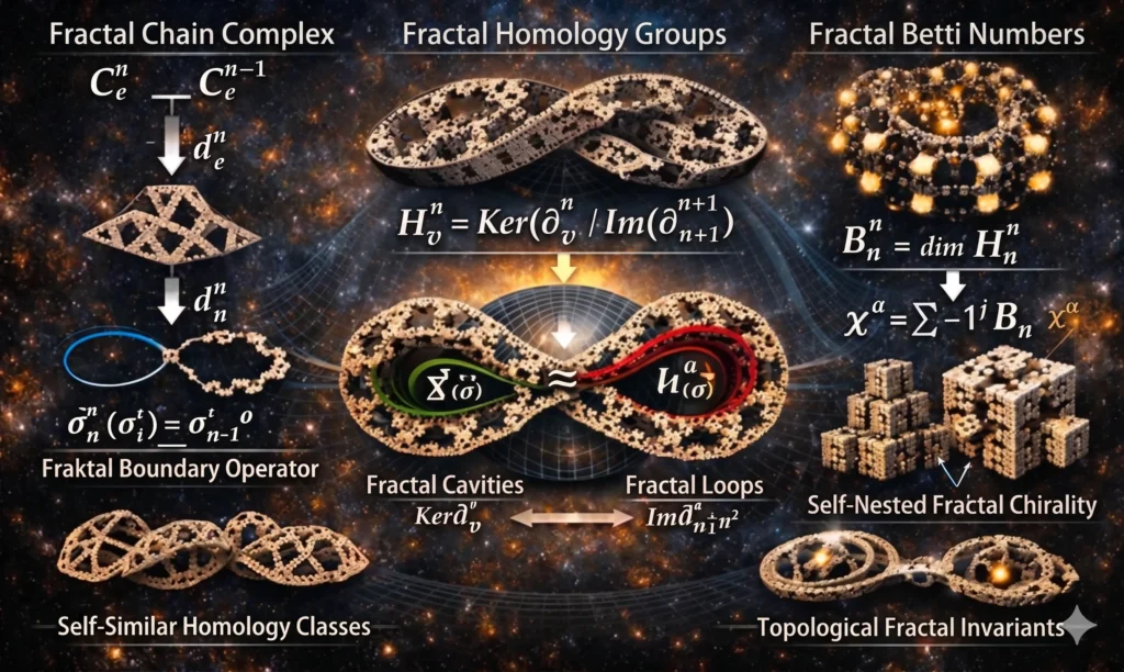
This infographic depicts the fractal extension of the classical homology concept—namely, the fractal redefinition of self-similar chains, boundary operators, and topological invariants.
On the left is the Fractal Chain Complex: a fractal boundary operator (∂𝑛Φ) descending from a Sierpinski tetrahedron-like structure toward a smaller Sierpinski triangle is shown. This symbolizes the transitionary boundary relationship of fractal chains. The Fractal Homology Groups section is in the center; fractal gaps and fractal loops are connected around the equation 𝐻𝑛Φ = Ker(∂𝑛Φ)/Im(∂𝑛+1Φ). On the right are Fractal Betti Numbers (𝐵𝑛Φ = dim 𝐻𝑛Φ) and Fractal Euler Characteristic (𝜒Φ = ∑(−1)𝑛𝐵𝑛Φ); these measure the degrees of connectivity and gaps in fractal topology.
The Self-Similar Homology Classes and Topological Fractal Invariants at the bottom visualize the multi-scale topological continuity of fractal chains. This structure is used to understand how homology groups evolve in a self-similar manner in fractal topology and how topological resonances are measured in quantum systems.
Fractal Initial Hilbert Space Visual
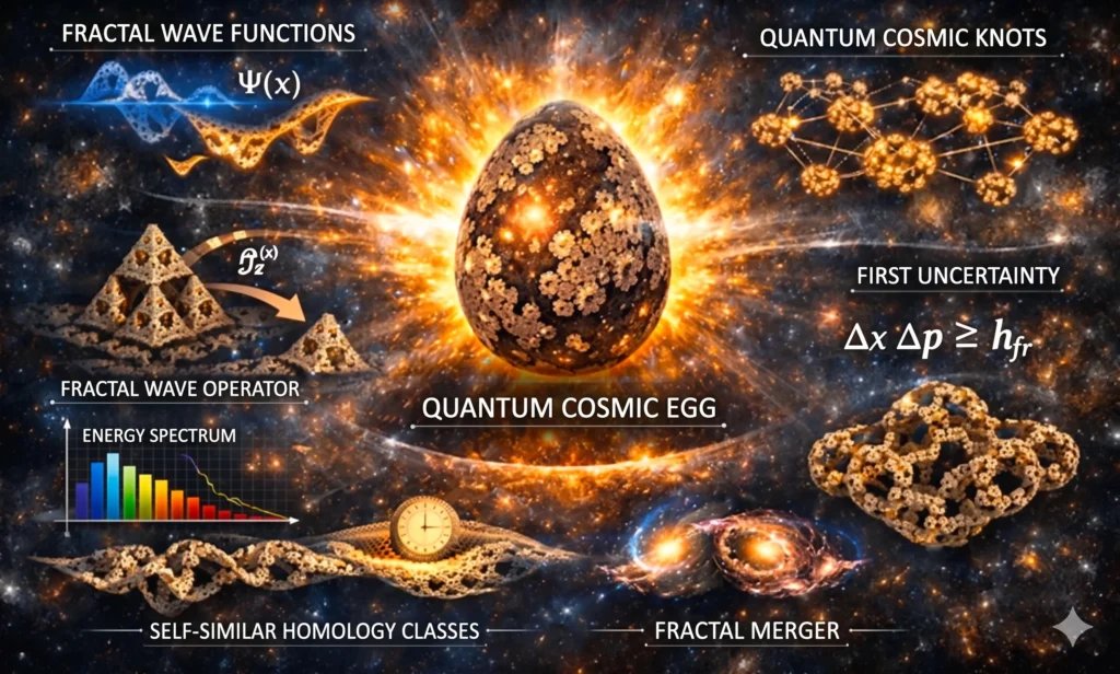
This illustration depicts the quantum origin and cognitive starting point of fractal Hilbert space.
The Quantum Cosmic Egg at the center symbolizes the first potential of the universe as an energy core covered with fractal patterns. While Fractal Wave Functions (Ψ(𝑥)) are in the top left corner, the Proto-Hilbert Field and energy spectrum are in the bottom left corner. Quantum Cosmic Knots at the top right show universal fractal connections; in the bottom right, the Initial Uncertainty (Δ𝑥 Δ𝑝 ≥ ℎfr) section represents the fractal quantum uncertainty principle.
The Initial History and Space and Fractal Unification labels at the bottom summarize the unification of the fractal universe with quantum consciousness. This structure is used to model the most fundamental structural level of the universe in the unification of fractal and quantum physics.