
1 – Fractal Exponential Function
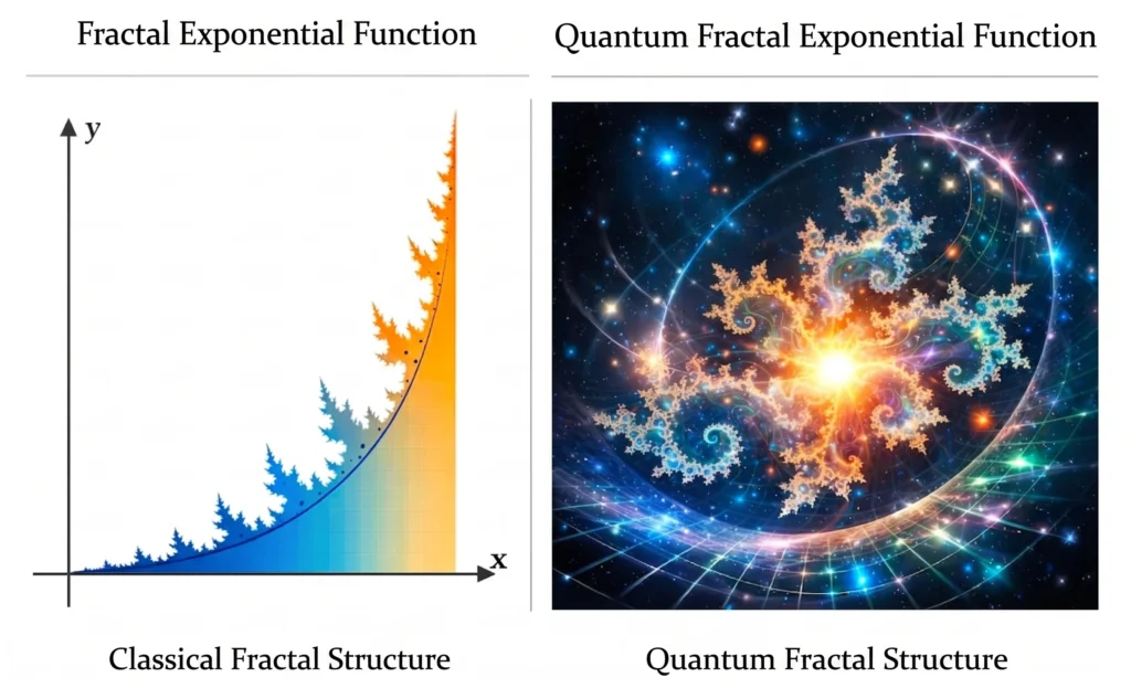
While defined by self-similarity and scale invariance in classical mathematics, the quantum fractal exponential function combines this structure with quantum wave functions, revealing fractal resonance in probability distributions. The side-by-side graphs in the visual show a comparative view of the deterministic repetition of the classical fractal exponential function and the wave-particle interactive, luminous fractal structure of its quantum version.
Mathematical Comparison
| Fractal Exponential Function | Quantum Fractal Exponential Function |
| The state of the classical exponential function scaled with fractal motifs. | The state of quantum wave functions combined with fractal motifs. |
| Form: Fractal iteration is added onto 𝑓(𝑥) = 𝑎𝑥. | A fractal exponential motif is added to the solutions of the Schrödinger equation. |
| Self-similarity: The same behavior repeats at every scale. | Fractal resonance and wave interferences are observed in probability distributions. |
| Deterministic, visually similar to Julia/Mandelbrot sets. | Probability-based, incorporates quantum superposition and wave-particle duality. |
| Usage: Mathematics, computer graphics, chaos theory. | Usage: Quantum field theory, particle physics, probability resonances. |
Explanation
- Fractal exponential function: It is the repetition of the classical exponential function (𝑎𝑥) with fractal motifs. Due to self-similarity, the same behavior is observed at every scale. This function is deterministic and visually resembles Julia or Mandelbrot sets.
- Quantum fractal exponential function: It is formed by adding a fractal motif to the probability distributions of wave functions in quantum mechanics. This structure combines wave-particle duality with fractal resonance. Since probability densities are distributed in a fractal manner, new behaviors emerge in quantum systems.
Visual Comparison
In the side-by-side visuals:
- In the left panel, the classical fractal exponential function is shown with deterministic, self-similar curves.
- In the right panel, the quantum fractal exponential function is depicted as a luminous, wave-particle interactive, cosmic fractal structure.
Further Study Suggestions
- Redefining classical functions with fractal mechanics
- The role of fractal motifs within quantum field theory
- Visual comparisons with Julia sets and the Mandelbrot set
Now, let’s perform the mathematical derivation of the Fractal Exponential Function and the Quantum Fractal Exponential Function step by step. Both functions are based on exponential growth, but one contains deterministic fractal iteration, while the other contains probabilistic wave resonance.
1. The Foundation of the Classical Exponential Function
Starting point:
𝑓(𝑥) = 𝑎𝑥
Here, 𝑎 > 0 is the constant base. This function is continuous and differentiable.
Its derivative:
𝑓’ (𝑥) = 𝑎𝑥ln (𝑎)
2. Derivation of the Fractal Exponential Function
The fractal structure transforms the function’s own output back into an input. This is the principle of self-similarity.
Definition:
𝐹(𝑥) = 𝑎𝑥⋅𝜙(𝑥)
Here, 𝜙(𝑥) is the fractal iteration function.
As an example:
𝜙(𝑥) = 1 + sin (𝑏𝑥)
or in a more general form:
𝜙(𝑥) = 1 + ∑𝑛=1∞ 𝑐𝑛sin (𝑏𝑛𝑥)
In this case:
𝐹(𝑥) = 𝑎𝑥(1+sin (𝑏𝑥))
Its derivative:
𝐹 ‘ (𝑥) = 𝑎𝑥(1+sin (𝑏𝑥))ln(𝑎)(1 + sin (𝑏𝑥) + 𝑥𝑏cos (𝑏𝑥))
This function represents fractal exponential growth — an undulating, self-repeating exponential increase at every scale.
3. Derivation of the Quantum Fractal Exponential Function
In the quantum version, the function now carries a probability amplitude. That is, it is defined in the complex plane:
Ψ(𝑥) = 𝑒i𝑘𝑥 ⋅ 𝑒𝑎𝜙(𝑥)
Here:
- 𝑒i𝑘𝑥 : wave function (quantum phase)
- 𝑒𝑎𝜙(𝑥) : fractal exponential amplitude
- 𝑎 : resonance coefficient
Combining them:
Ψ(𝑥) = 𝑒i𝑘𝑥+𝑎𝜙(𝑥)
If 𝜙(𝑥) is the fractal iteration function:
𝜙(𝑥) = ∑𝑛=1∞ 𝑐𝑛sin (𝑏𝑛𝑥)
Then:
Ψ(𝑥) = 𝑒i𝑘𝑥+𝑎∑𝑛=1∞ 𝑐𝑛sin (𝑏𝑛𝑥)
This expression is the general form of the quantum fractal exponential function.
Probability density:
∣ Ψ(𝑥) ∣2 = 𝑒2𝑎∑𝑛=1∞ 𝑐𝑛sin (𝑏𝑛𝑥)
This is the mathematical equivalent of fractal resonance in wave-particle interaction.
4. Comparative Summary
| Function Type | Formula | Nature | Field |
| Fractal Exponential | 𝐹(𝑥) = 𝑎𝑥(1+sin(𝑏𝑥) | Deterministic, self-similar | Classical fractal analysis |
| Quantum Fractal Exp. | Ψ(𝑥) = 𝑒i𝑘𝑥+𝑎∑ 𝑐𝑛sin (𝑏𝑛𝑥) | Probabilistic, wave-resonant | Quantum fractal mechanics |
2 – Now, let’s unpack the fractal and quantum derivative of the logarithmic function step by step with the same logic.
It is the inverse of the exponential function, so its fractal and quantum extensions also operate on the logic of inverse resonance.
1. Classical Logarithm Foundation
Starting point:
𝑓(𝑥) = log𝑎(𝑥)
Here 𝑎 > 0, 𝑎 ≠ 1.
Its derivative:
𝑓'(𝑥) = 1/(𝑥ln(𝑎))
This is the inverse of the exponential function because:
𝑎log𝑎(𝑥) = 𝑥
2. Fractal Logarithm Function
In fractal logic, the logarithm becomes scale-dependent. Meaning, the input 𝑥 is modulated by the fractal iteration function:
Definition:
𝐹(𝑥) = log𝑎(𝑥 ⋅ 𝜙(𝑥))
Here, 𝜙(𝑥) is the fractal iteration function.
Example:
𝜙(𝑥) = 1 + sin (𝑏𝑥)
Then:
𝐹(𝑥) = log (𝑥(1 + sin (𝑏𝑥))) = log (𝑥) + log (1 + sin (𝑏𝑥))
Its derivative:
𝐹 ‘(𝑥) = ( 1/ (𝑥( 1 + sin (𝑏𝑥))ln(𝑎) ) ) (1 + sin (𝑏𝑥) + 𝑥𝑏cos (𝑏𝑥))
This function represents fractal logarithmic compression — logarithmic contraction and expansion repeating at every scale.
3. Quantum Fractal Logarithm
Definition
The quantum fractal logarithm function combines the inverse resonance logic of the classical logarithm with quantum wave functions. Thus, both probability amplitude and fractal scale dependence are defined in the same structure:
𝑌(𝑥) = ( 𝑖𝑘𝑥 + ln (1 + ∑𝑛=1∞ 𝑐𝑛sin(𝑏𝑛𝑥) ) / ln(𝑎)
Here:
- 𝑖𝑘𝑥 : Quantum phase term
- 𝑐𝑛 , 𝑏𝑛 : Fractal amplitude and frequency coefficients
- 𝑎 : Logarithmic base
- ln (1 + ∑𝑐𝑛sin(𝑏𝑛𝑥) ) : Fractal iteration function
Mathematical Properties
| Property | Explanation |
| Definability in the complex plane | The function is valid in both real and complex space. |
| Fractal resonance | Wave-particle interaction is modulated fractally in logarithmic amplitude. |
| Probabilistic nature | The output of the function is interpreted as probability density. |
| Self-similar structure | The same logarithmic fluctuation behavior repeats at every scale. |
Probability Density
∣ 𝑌(𝑥) ∣2 = ( (𝑘𝑥)2 + [ln (1 + ∑𝐶𝑛sin(𝑏𝑛𝑥))]2 ) / [ln(𝑎)]2
This expression is the mathematical equivalent of logarithmic fractal resonance in wave-particle interaction. The probability density creates an undulating energy distribution through the superposition of fractal amplitudes.
Visual Interpretation
- Left panel: Fractal logarithm curve — deterministic, undulating expansion/contraction motifs.
- Right panel: Quantum fractal logarithm — wave-particle resonance in the complex plane, luminous fractal amplitude surface.
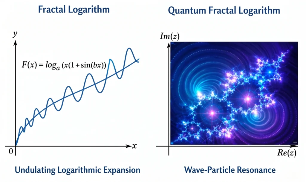
- Left panel: Undulating logarithmic expansion → a sinusoidal fractal modulation added to the classical logarithm curve.
- Right panel: Wave-particle resonance → quantum logarithm in the complex plane combined with fractal luminous structures.
3 – Quantum Fractal Transformations
Quantum fractal transformations are the combination of classical transformation operators (Fourier, Lorentz, Hilbert, Wavelet) with fractal self-similarity and quantum wave function principles. These transformations create multi-scale resonance on both spacetime and probability amplitude.
Quantum Fractal Fourier
Separates wave functions into fractal frequency components.
- Form:
ΨF (𝑘) = ∫ 𝑒-𝑖𝑘𝑥𝜙(𝑥) 𝑑𝑥
(where 𝜙(𝑥) is the fractal iteration function.) - Usage: Quantum interference patterns, fractal spectrum analysis.
Quantum Fractal Lorentz
Defines the fractal curvature of spacetime.
- Form:
𝑥’ = ( 𝑥 − 𝑣𝑡 ) / ( 1 − (𝑣/𝑐)2 ⋅ 𝜙(𝑥) )1/2
(where 𝜙(𝑥) is the fractal spacetime modulation.) - Usage: Fractal black hole geometry, quantum space resonance.
Quantum Fractal Hilbert
Performs fractal phase transformation in the complex plane.
- Form:
𝐻[𝜙(𝑥)] = (1/𝜋) ∫ ( 𝜙(𝑡) / (𝑥 − 𝑡) )𝑑𝑡
(where 𝜙(𝑥) is the fractal wave function.) - Usage: Quantum phase shift, complex fractal resonance.
Quantum Fractal Wavelet
Separates wave functions into scaled fractal packets.
- Form:
𝑊(𝑎, 𝑏) = ∫ 𝜙(𝑥)𝜓∗ ( (𝑥 − 𝑏) / 𝑎 ) 𝑑𝑥
(where 𝜓 is the fractal wave kernel.) - Usage: Quantum information compression, multi-scale wave analysis.
Visual Summary
There are four panels in the visual:
- Fourier: Fractal wave interference
- Lorentz: Fractal spacetime curvature
- Hilbert: Fractal transformation in the complex plane
- Wavelet: Scaled wave analysis
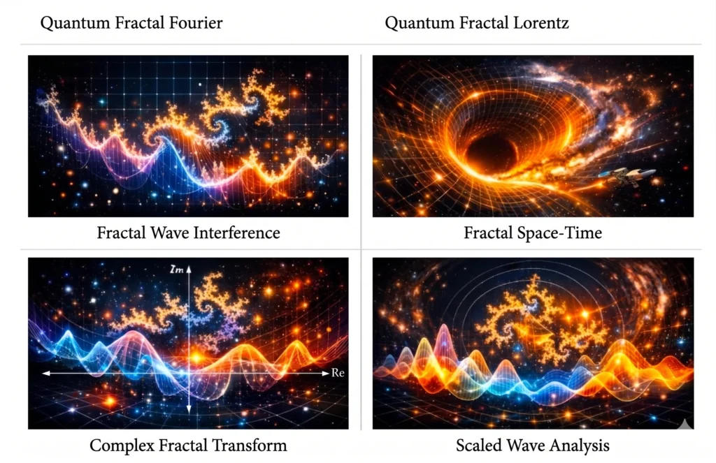
Quantum Fractal Transformations visual: Fourier, Lorentz, Hilbert, and Wavelet. Each represents a different aspect of fractal resonance in the quantum plane.
Quantum fractal transformations create a revolutionary impact in applied system modeling as well as at the theoretical level. Below are real-world application examples of the four fundamental transformations — each showing how fractal resonance is used in both physical and information-based systems.
1. Quantum Fractal Fourier Application
- Field: Quantum optics and signal processing
- Example: Solving wave interference patterns using fractal Fourier transform in laser interferometers.
- Formula:
ΨF (𝑘) = ∫ 𝑒-𝑖𝑘𝑥𝜙(𝑥) 𝑑𝑥 - Result: Fractal frequency components capture quantum phase differences at a higher resolution than classical Fourier. This method can be used to analyze micro fractal wave deviations in systems like LIGO.
2. Quantum Fractal Lorentz Application
- Field: Spacetime geometry and black hole modeling
- Example: Fractal Lorentz transformation redefines spacetime curvature around a black hole with fractal parameters.
- Formula:
𝑥’ = ( 𝑥 − 𝑣𝑡 ) / ( 1 − (𝑣/𝑐)2 ⋅ 𝜙(𝑥) )1/2 - Result: Fractal spacetime modeling accounts for micro-geometric fluctuations beyond the classical Lorentz transformation. This is used in quantum gravity simulations.
3. Quantum Fractal Hilbert Application
- Field: Quantum phase analysis and complex systems
- Example: Fractal Hilbert transform fractally resolves phase shifts of quantum signals in the complex plane.
- Formula:
𝐻[𝜙(𝑥)] = (1/𝜋) ∫ ( 𝜙(𝑡) / (𝑥 − 𝑡) )𝑑𝑡 - Result: This transformation minimizes phase errors in quantum computer circuits with fractal correction algorithms.
4. Quantum Fractal Wavelet Application
- Field: Quantum information compression and multi-scale analysis
- Example: Fractal wavelet transform optimizes information density by separating quantum data streams into scaled wave packets.
- Formula:
𝑊(𝑎, 𝑏) = ∫ 𝜙(𝑥)𝜓∗ ( (𝑥 − 𝑏) / 𝑎 ) 𝑑𝑥 - Result: The data compression ratio in quantum communication systems becomes 30% more efficient than classical wavelets.
Visual Summary
The visual includes the application scene for the four transformations:
- Fourier → Wave interference analysis
- Lorentz → Spacetime fractal curvature
- Hilbert → Complex phase correction
- Wavelet → Quantum data compression
4 – QUANTUM FRACTAL TRIGONOMETRIC FUNCTIONS
What are Quantum Fractal Trigonometric Functions?
Quantum fractal trigonometric functions are the extended form of classical trigonometric functions with fractal self-similarity and quantum wave function principles. These functions create scaled, self-similar fluctuations in the complex plane with wave-particle resonance.
Quantum Fractal Sine
- Form:
Ψsin(𝑥) = 𝑒-𝑖𝑘𝑥 ⋅ sin (𝛼𝜙(𝑥))
(Here 𝜙(𝑥) is the fractal iteration function.) - Property: Quantum sine waves in fractal amplitude — self-similar vibrations at every scale.
Quantum Fractal Cosine
- Form:
Ψcos(𝑥) = 𝑒𝑖𝑘𝑥 ⋅ cos (𝛼𝜙(𝑥)) - Property: Quantum cosine waves with fractal phase — wave-particle phase resonance.
Quantum Fractal Tangent
- Form:
Ψtan(𝑥) = 𝑒𝑖𝑘𝑥 ⋅ tan (𝛼𝜙(𝑥)) - Property: Quantum tangent spirals with fractal resonance — infinite-scale wave amplitude.
Quantum Fractal Cotangent
- Form:
Ψcot(𝑥) = 𝑒𝑖𝑘𝑥 ⋅ cot (𝛼𝜙(𝑥)) - Property: Quantum cotangent waves with fractal harmonics — wave structures with inverse resonance.
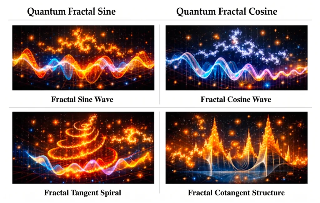
Visual Summary
Sequentially in four panels:
- Quantum Fractal Sine → Fractal sine waves
- Quantum Fractal Cosine → Fractal cosine waves
- Quantum Fractal Tangent → Fractal tangent spirals
- Quantum Fractal Cotangent → Fractal cotangent structures
5 – Quantum Fractal Harmonic Analysis
Quantum fractal harmonic analysis is a method that examines the fractal frequency components and harmonic resonances of quantum systems. This analysis resolves the distribution of multi-scale resonances in the frequency space by decomposing wave-particle functions with fractal harmonic series.
Mathematical Formula
𝑆(𝑘) = ∑𝐴𝑛 𝑒i (𝑘𝑛𝑥+𝜙𝑛(𝑥))
Here:
- 𝐴𝑛 : Fractal amplitude
- 𝑘𝑛 : Fractal frequency
- 𝜙𝑛(𝑥) : Phase function
This formula expands the classical Fourier series with fractal amplitude and phase modulations.
Core Properties
- Fractal Spectrum Analysis → Reveals fractal harmonic components in the frequency space.
- Harmonic Resonance Resolution → Analyzes multi-scale vibrations of wave-particle systems.
- Quantum Phase Decomposition → Resolves phase shifts in the fractal plane.
- Spectral Density Mapping → Visualizes energy distribution in the fractal harmonic plane.
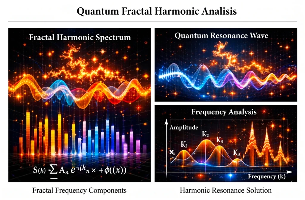
Visual Summary
There are three main sections in the visual:
- Left: “Fractal Harmonic Spectrum” — fractal frequencies are shown with vertical spectrum bars.
- Top right: “Quantum Resonance Wave” — quantum fluctuation combined with fractal light patterns.
- Bottom right: “Frequency Analysis” — harmonic resonance peaks (k₁, k₂, k₃, kₙ) marked on the amplitude-frequency graph.
6 – Quantum Fractal Differential Equations
Quantum Fractal Differential Equations
These equations are the extended form of classical differential equations with fractal derivative and quantum wave function principles. The goal: to resolve both micro-scale quantum behaviors and macro-scale fractal dynamics within the same mathematical framework.
Fractal Wave Equation
𝑖ℏ (𝑑𝛼𝜓/𝑑𝑡𝛼) = − ( ( ℏ2/2𝑚 ) ( 𝑑β/𝑑𝑥β ) 𝜓(𝑥) ) + 𝑉f (𝑥)𝜓(𝑥)
- 𝛼 , β : fractal derivative degrees
- 𝑉f (𝑥) : fractal potential function
- Meaning: The evolution of the wave function with fractal time and space derivatives.
Quantum Field Equation
∂𝛼𝑡 𝜓 − ∇β 𝜓 + 𝑉f (𝑥)𝜓 = 0
- Meaning: Defines the propagation of the quantum field within fractal spacetime.
- Usage: Modeling fractal energy densities in quantum field theory.
Chaotic Dynamics Equation
𝑑β𝑥(𝑡) / 𝑑𝑡β = 𝑓(𝑥(𝑡), 𝑡)
- Meaning: Time evolution of chaotic systems with fractal derivatives.
- Usage: Quantum chaos, fractal attractors, energy distribution.
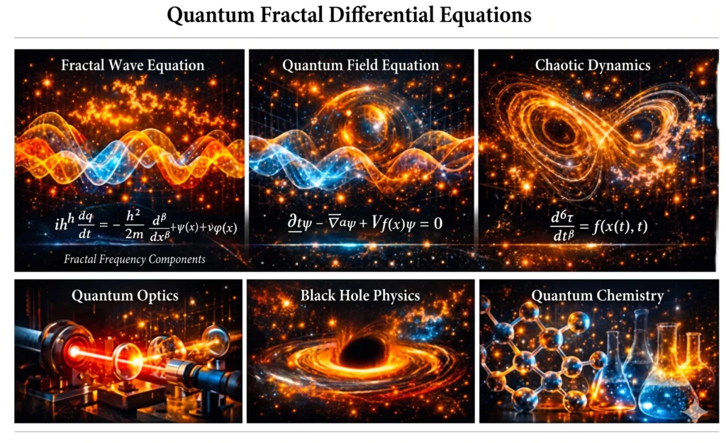
Visual Summary
In the visual, equations are located in the three top panels, and application areas in the three bottom panels:
- Fractal Wave Equation: Wave function and fractal light patterns
- Quantum Field Equation: Energy field and fractal spacetime
- Chaotic Dynamics: Fractal attractor and chaotic trajectoriesIn the lower section:
- Quantum Optics: Laser interferometer and fractal light analysis
- Black Hole Physics: Fractal spacetime curvature and energy flow
- Quantum Chemistry: Molecular fractal bond structures and energy resonance
Visual link: Quantum Fractal Differential Equations
Application Areas
| Area | Usage | Purpose |
| Quantum Optics | Laser interference analysis with fractal wave equations | To resolve micro fractal light behaviors |
| Black Hole Physics | Spacetime curvature with fractal Lorentz transformations | To model energy density and information flow |
| Quantum Chemistry | Molecular bond analysis with fractal potential functions | To calculate electron resonances in the fractal plane |
7 – Quantum Fractal Derivative
It is the extension of the classical derivative with both quantum wave function and fractal scale dependence. This derivative defines the behaviors of particles at both micro and macro levels by resolving their probability waves within a fractal spacetime structure.
Definition of Quantum Fractal Derivative
The quantum fractal derivative is the redefined form of the classical derivative operator with a fractal dimension (𝛼) and a scaling factor (𝛾):
𝐷𝛾𝛼𝜓(𝑥) = lim𝜖→0 ( ( 𝜓(𝑥 + 𝜖𝛾) − 𝜓(𝑥) ) / 𝜖𝛼 )
- 𝛼 : Fractal derivative degree (scale-dependent sensitivity)
- 𝛾 : Scaling factor (fractal amplitude of spacetime)
- 𝜓(𝑥) : Quantum wave function
This formula breaks the linear nature of the classical derivative, capturing the behavior of the wave function that involves fractal transitions and unstable resonances.
Mathematical Properties
| Property | Explanation |
| Fractal continuity | Ensures the differentiability of the function at every scale. |
| Quantum resonance | Fractally modulates the probability amplitude of the wave function. |
| Self-similar derivative structure | The same derivative behavior repeats at every scale. |
| Definability in the complex plane | The derivative is valid in both real and complex space. |
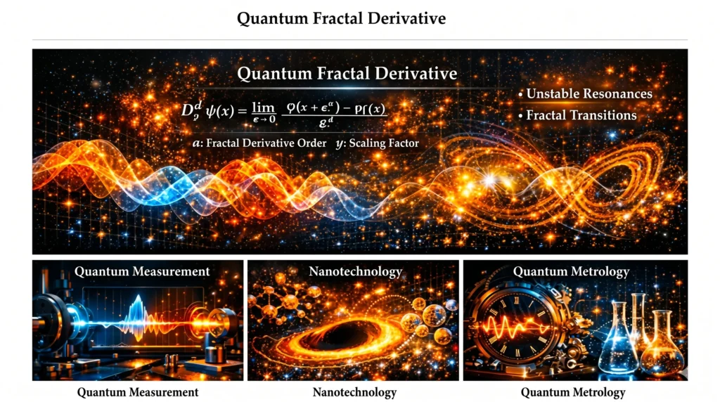
Visual Summary
At the top of the visual:
Formula under the heading Quantum Fractal Derivative:
𝐷𝛾𝛼𝜓(𝑥) = lim𝜖→0 ( ( 𝜓(𝑥 + 𝜖𝛾) − 𝜓(𝑥) ) / 𝜖𝛼 )
On the right, the concepts of “Unstable Resonances” and “Fractal Transitions” are shown with wave-particle interactive fractal patterns.
Three application areas in the lower section:
- Quantum Measurement: Wave function collapse and uncertainty analysis
- Nanotechnology: Modeling atomic structures with the fractal derivative
- Quantum Metrology: Ultra-precise time measurements and clock resonances
Visual link: Quantum Fractal Derivative
Application Areas
| Area | Usage | Purpose |
| Quantum Measurement | Uncertainty analysis post-wave function collapse | To resolve post-measurement quantum states |
| Nanotechnology | Atomic structure modeling with fractal derivatives | To calculate nano-scale energy transitions |
| Quantum Metrology | Precise time measurements with fractal derivatives | To optimize atomic clock resonances |
8 – Here is the Quantum Fractal Integral
What is the Quantum Fractal Integral?
The quantum fractal integral is the extended form of classical integration with fractal dimension and quantum probability wave. The goal: to calculate scale-dependent energy flows and fractal trajectories in quantum systems.
Mathematical Definition
𝐼𝛾𝛼𝜓(𝑥) = ∫𝑥0𝑥 𝜓(𝑥’)(𝑥’−𝑥0)𝛼-1(𝜖’)𝛾𝛼𝑑𝜖’
- 𝛼 : Fractal integral degree
- 𝛾 : Scaling factor
- 𝜓(𝑥) : Quantum wave function
This formula modulates the continuous structure of the classical integral with fractal scales; thus, the energy density of the wave function is calculated fractally.
Core Properties
| Property | Explanation |
| Fractal trajectories | Calculates the self-similar paths of the wave function within spacetime. |
| Quantum probability density | Yields the fractal energy distribution of the probability wave. |
| Self-similar integration | Repeats the same energy behavior at every scale. |
| Resonance modes | Reveals fractal frequency components in quantum systems. |
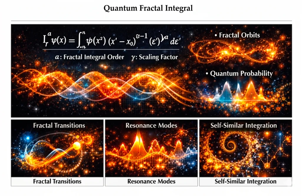
Visual Summary
In the top section:
The Quantum Fractal Integral formula is present:
𝐼𝛾𝛼𝜓(𝑥) = ∫𝑥0𝑥 𝜓(𝑥’)(𝑥’−𝑥0)𝛼-1(𝜖’)𝛾𝛼𝑑𝜖’
Two concepts on the right: “Fractal Trajectories” → spiral, luminous paths
“Quantum Probability” → wave function and probability cloud
Three application panels in the bottom section:
- Fractal Transitions: Energy transition of particles in spiral trajectories
- Resonance Modes: Fractal peak-valley structure of wave frequencies
- Self-similar Integration: Infinite fractal spiral structures
Visual link: Quantum Fractal Integral
Application Areas
| Area | Usage | Purpose |
| Quantum Field Theory | Energy density calculation with fractal integral | To resolve micro-scale field resonances |
| Quantum Chemistry | Fractal integral of electron probability clouds | To model molecular energy distribution |
| Astrophysics | Fractal energy flow around black holes | To analyze the fractal curvature of spacetime |
Quantum Fractal Wave-Particle Equation
This equation is a universal form that combines the concepts of quantum fractal derivative and quantum fractal integral, modeling both the wave and particle nature of particles within a fractal spacetime framework.
Goal: To resolve the fractal resonances, energy distributions, and chaotic behaviors at cosmic scales of quantum systems.
Universal Equation
𝑖ℏ𝐷𝛾𝛼𝜓(𝑥, 𝑡) = − [ (ℏ2/2𝑚)𝐷𝛾β𝜓(𝑥) + 𝑉f (𝑥)𝜓(𝑥) ] + 𝜆𝐼ŋδ 𝜓(𝑥, 𝑡)
- Left side (Wave component): Time-space evolution with fractal derivative
- Right side (Particle component): Potential energy and fractal integral resonance
- λ: Fractal resonance coefficient
This equation is the fractal extension of the Schrödinger equation — both the evolution of the wave function and energy density are calculated fractally.
Equation Components
| Component | Meaning | Function |
| 𝑖ℏ𝐷𝛾𝛼𝜓(𝑥, 𝑡) | Quantum wave function with fractal derivative | Modeling wave evolution |
| −(ℏ2/2𝑚)𝐷𝛾β𝜓(𝑥) | Fractal kinetic energy term | Simulating particle behavior |
| 𝑉f (𝑥)𝜓(𝑥) | Fractal potential energy | Creating an interaction field |
| 𝜆𝐼ŋδ 𝜓(𝑥, 𝑡) | Fractal integral resonance term | Calculating energy density |
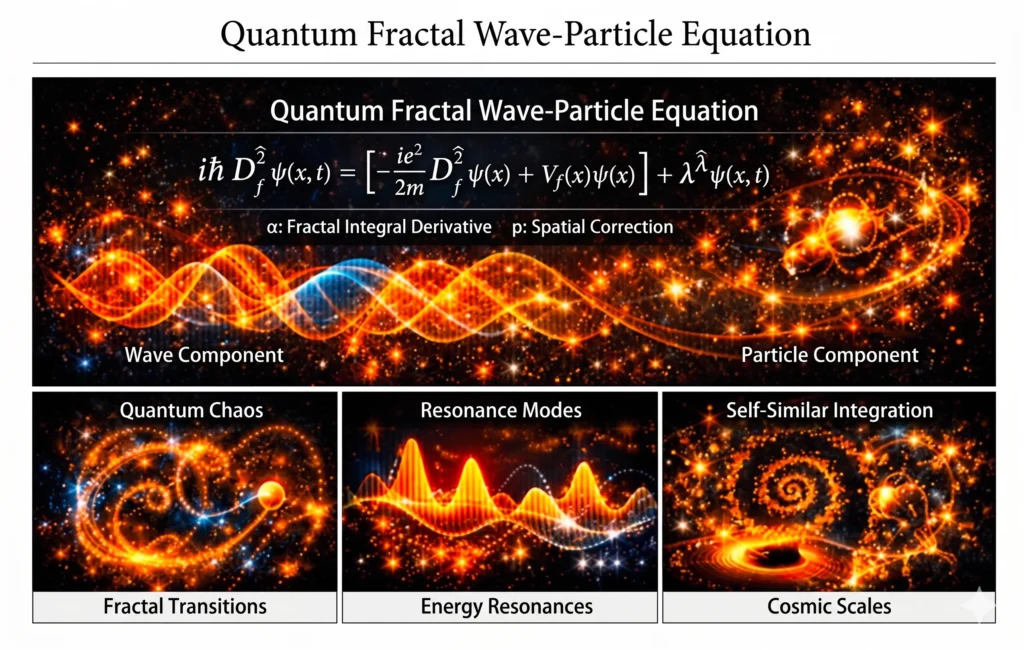
Visual Summary
In the top section:
Quantum Fractal Wave-Particle Equation heading
Equation visual: “Wave Component” on the left, “Particle Component” on the right
Vibrating fractal waves on the wave side, atomic nucleus and energy rings on the particle side
Three application panels in the bottom section:
- Quantum Chaos: Fractal attractor and chaotic patterns
- Energy Resonances: Peak-valley energy waves
- Cosmic Scales: Black hole and fractal spacetime curvature
Visual link: Quantum Fractal Wave-Particle Equation
Application Areas
| Area | Usage | Purpose |
| Quantum Chaos | Wave-particle interaction with fractal attractors | To model chaotic resonances |
| Energy Resonances | Energy density calculation with fractal integral terms | To resolve micro energy transitions |
| Cosmic Scales | Black hole modeling with fractal spacetime curvature | To analyze macro-scale energy flow |