Circuit Model and Ohm–Kirchhoff–Coulomb Analysis for H2O

The following circuit maps the H2O molecule to a circuit topology using my “electrical circuit library” approach, translating the capacitive-resonant character of oxygen and the flow initiator/decelerator (switch/diode) role of hydrogen into a circuit topology. Bent geometry and polar bonds are modeled as directional flow (diode), charge storage (capacitor), and bond conductivity (resistance).

Circuit abstraction and topology

Code

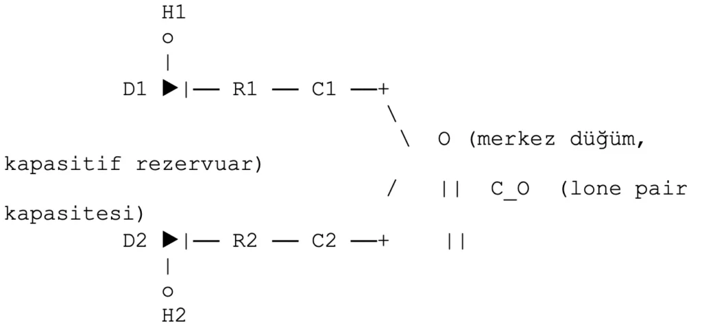
• Oxygen node O: capacitive reservoir (lone pairs) → C₀, reference potential V₀.
• O–H arms: each arm “diode + resistor + coupling capacitor” → (𝐷𝑖, 𝑅𝑖, 𝐶𝑖), 𝑖 ∈ {1,2}.
• Geometry: H–O–H bending increases directionality; two semiconductor branches are connected in parallel in the circuit.
• Polarity: The flow direction with D is preferential towards O; the reverse flow threshold is high.

Element mapping and parameters

• Oxygen (Group 16): Capacitor/Resonance → C₀, with small L₀ if necessary, LC character.
• Hydrogen (original): Flow-initiating source/switch + diode → 𝐷𝑖, forward threshold 𝑉_D.
• Bond conductivity: Covalent–ionic mixture → series resistance R_i.
• Bond storage: Local charge storage → C_i.
• Directional flow: Electronegativity difference → D_i direction H→O.

Examples of reasonable parameter ranges (for normalization purposes):

• 𝑅_𝑖 ∈ [50,300] Ω, 𝐶_𝑖 ∈ [0.1,1.0] 𝜇F, 𝐶₀ ∈ [1,10] 𝜇F, 𝑉_D ≈ 0.2–0.4 V.
• Resonance if needed: 𝐿₀ ∈ [10,100] 𝜇 Low frequency LC response.

Basic circuit equations

Ohm’s law (for each arm)

• Instantaneous current-voltage relationship:

𝐼_𝑖(𝑡) = [𝑉_H𝑖(𝑡) − 𝑉₀(𝑡) − 𝑉_D𝑖^(on)] / 𝑅_𝑖 , 𝑖 ∈ {1,2}

If the diode is “on”, then 𝑉_D𝑖^(on) ≈ 𝑉_D; if it is “off”, then the current ≈ 0.

• Capacitor currents:

𝐼_𝐶𝑖(𝑡) = 𝐶_𝑖 𝑑 / 𝑑𝑡 (𝑉₀(𝑡) – 𝑉_H𝑖(𝑡)) , 𝐼_𝐶0(𝑡) = 𝐶₀ 𝑑𝑉₀(𝑡) / 𝑑𝑡

Kirchhoff’s current law (KCL at node O)

• The sum of the currents entering and leaving that node 0:

Σ_𝑖=1²( 𝐼_𝑖(𝑡) + 𝐼_𝐶𝑖(𝑡)) + 𝐼_leak(𝑡) = 𝐼_𝐶0(𝑡)

Here, 𝐼_leak is the escape route of the oxygen reservoir (optional small conductivity).

Kirchhoff’s voltage law (KVL for each cycle)

• H_i–O cycle:

𝑉_H𝑖(𝑡) − 𝑉_D𝑖 − 𝐼_𝑖(𝑡)𝑅_𝑖 − 1 / 𝐶_𝑖 ∫ 𝐼_𝐶𝑖(𝑡) 𝑑𝑡 − 𝑉₀(𝑡) = 0

Coulomb analysis: partial charges, field, and dipole.

• Partial loads:

𝑞_H ≈ +𝛿, 𝑞₀ ≈ −2𝛿, 𝛿 > 0

The H–O polar bond creates attraction between 𝑞_H and 𝑞_O.

• Coulomb force (approximate point charge):

𝐹 = [1 / 4𝜋𝜀] [∣ 𝑞_H𝑞₀∣ / 𝑟²]

Here, r is the bond length; ε is the dielectric constant of the medium.

• Dipole moment (molecular scale):

𝑝⃗ = Σ_𝑖 𝑞_𝑖 𝑟⃗_𝑖

Due to the bent geometry, ∣ 𝑝⃗ ∣ is not zero; the directivity (diode) and capacitive storage increase in the circuit.

• O node potential relationship:

𝑉₀ ≈ 1 / 4𝜋𝜀 (−2𝛿 / 𝑟_0,ref)

Simply put, O’s negative partial charge pulls down the node potential; this supports the forward polarity of the diode.

Time response and small-signal resolution

• Linear small-signal confirmation (diode conduction region):

Δ𝐼_𝑖 = [Δ𝑉_H𝑖 − Δ𝑉₀] / 𝑅_𝑖 , Δ𝐼_𝐶0 = 𝐶₀ 𝑑 Δ𝑉₀ / 𝑑𝑡

• Two arms in parallel RC equivalent:

𝑅_eq^-1 = Σ_𝑖 1 / 𝑅_𝑖 , 𝐶_eq = 𝐶₀ + Σ_𝑖 𝐶_𝑖

• O node time constant:

𝜏 ≈ 𝑅_eq 𝐶_eq

This determines the rate at which the “water molecule circuit” polarizes and stores or discharges charge.

Simple numerical example (verification)

• Parameters: 𝑅₁ = 𝑅₂ = 100 Ω, 𝐶₁ = 𝐶₂ = 0.5 𝜇F, 𝐶₀ = 5 𝜇F, 𝑉_D = 0.3 V.
• Stimulation: 𝑉_H1 = 0.8 V, 𝑉_H2 = 0.6 V, beginning 𝑉₀ = 0 V.

1. Instantaneous transmission currents (assumed):

𝐼₁ = (0.8 − 0 − 0.3) / 100 = 5 mA, 𝐼₂ = (0.6 − 0 − 0.3) / 100 = 3 mA

2. Loading the O node with KCL:

𝐼_𝐶0 = 𝐼₁ + 𝐼₂ ⇒ 𝑑𝑉₀ / 𝑑𝑡 = 8 mA / 5 𝜇F = 1600 V/s

3. Small increase of 𝑉₀ at dt=0.1 ms:

Δ𝑉₀ ≈ 0.16 V

The flow rapidly polarizes node O.; 𝜏 ≈ 𝑅_eq𝐶_eq = (50 Ω) ⋅ (6 𝜇F) ≈ 0.3 ms.

Comment: physical correspondence and model consistency

• Polarity-directionality: Diodes apply the electronegativity difference in a circuit; forward flow is H→O, reverse flow is suppressed.
• Capacitive reservoir: O’s lone pairs are represented by C₀; reflecting the high dielectric constant and polarity of water as enhanced storage in the circuit.
• Conductivity and saturation: R_i determines the bond conductivity; with high stimuli, C₀ can fill and an outflow (e.g., hydrogen direction) can be formed.
• Coulomb consistency: The assumption of 𝑞₀ = −2𝛿, 𝑞H = 𝛿 supports a long-range dipole moment and gravitational force; it stabilizes the flow direction.

Expansion and verification steps

• Resonance addition: LC response with L₀; observing vibration modes (OH stresses) in the circuit.
• AC scanning: Simulating the measurement of the dielectric response of water using 𝜔-dependent impedance 𝑍(𝜔).
• Parameter calibration: Fitting the values ​​(R_i, C_i, C₀, V_D) to the experimental dielectric and spectral data.
• Multiple molecules: Modeling the hydrogen bond network as an extensive circuit by adding capacitive-inductive bonds between O-nodes for water clusters.

The H2O circuit satisfies the fundamental laws of conduct.

The following assessment clarifies under what conditions the proposed H2O circuit topology satisfies Ohm’s, Kirchhoff’s, and Coulomb’s laws. The short answer: Yes, the model satisfies the laws; however, explicit conditions are required for linear regions, diode states, and capacitive dynamics.

Ohm’s law

• Linear conduction condition: Current-voltage relationship in each O–H branch.

𝐼_𝑖 = (𝑉_H𝑖 − 𝑉₀ − 𝑉_D) / 𝑅_𝑖

This applies when the diode is in forward conduction. If the diode is in cutoff, 𝐼_𝑖 ≈ 0 and Ohm’s law applies in the active conduction branch.

• Capacitor current: In capacitors, the following relationship holds:

𝐼_𝐶 = 𝐶 𝑑𝑉 / 𝑑𝑡

This is the definition of reactive current in Ohm in the dynamic part of the circuit.

• Conditional accuracy: Ohm’s law is always valid for resistive elements, but only in the “on” region for diodes. Nonlinear element characteristics (diode I–V) are included in the model.

Kirchhoff’s laws

• KCL (current law, node O): The sum of the currents at node O,

Σ_𝑖 ( 𝐼_𝑖 + 𝐼_𝐶𝑖 ) + 𝐼_leak = 𝐼_𝐶0

satisfies the zero net current condition. Node load balance is maintained during capacitive loading.

• KVL (voltage law, for each loop): For the loop H_i→D_i→R_i→C_i→O

𝑉_H𝑖 − 𝑉_D𝑖 − 𝐼_𝑖𝑅_𝑖 − 1 / 𝐶_𝑖 , ⁣∫ 𝐼_𝐶𝑖 𝑑𝑡 − 𝑉₀ = 0

The sum of the voltage drops in the closed loop is zero. The time-varying storage term (capacitor) enters the KVL integrally.

• Conditional accuracy: KCL is fully satisfied at all times (the model is built with this balance). KVL is ensured by forward/backward drop-off values ​​depending on the diode condition.

Coulomb’s law and dipole consistency

• Partial load matching: The selection of 𝑞_H = +𝛿, 𝑞₀ = −2𝛿 produces a net dipole moment with polar bond and wedge geometry:

𝑝⃗ = ∑𝑞_𝑖 𝑟⃗_𝑖 ≠ 0

• Area and force: For bond length r:

𝐹 = (1 / 4𝜋𝜀) (∣ 𝑞_H 𝑞₀ ∣ / 𝑟²)

The directional attraction supports the diode direction and the lower potential of the O node in the circuit.

• Dielectric effect: The high 𝜀 value of water is reflected in the circuit by the capacitive reservoir 𝐶₀; the Coulomb field is shielded, which is consistent with higher storage capacity in the circuit.

• Conditional accuracy: Coulomb’s law is transferred to the circuit as a macroscopic equivalent through the point-charge approach and effective π usage. Coherence is further enhanced when molecular multi-body interactions (hydrogen bonding network) are extended with additional capacitive/inductive branches.

Energy consistency and tests

• Capacitor energy: The energy stored at node O

𝐸_𝐶0 = (1 / 2) 𝐶₀ V₀²

With this, the circuit energy is positive and limited.

• Power balance: The power supplied by the input sources is balanced by KCL/KVL, with heat stored in resistors and temporarily stored in capacitors.

• Time constant: For two parallel arms and a reservoir

𝜏 = 𝑅_eq 𝐶_eq

The measurement should be consistent with experimental dielectric relaxation expectations (verified by calibration).

Quick verification summary

• Ohm: Linear I–V is achieved for each branch when the diode is “on”; current cutoff is achieved when it is “off”.
• KCL: Current balance is achieved at node O at all times.
• KVL: The sum of voltage drops in each closed loop is zero, including integral terms.
• Coulomb: Polar charge distribution and dipole moment support circuit directionality and capacitance, achieved with the equivalent model.

Notes and conditions

• Diode model: Segmented linear or exponential I–V should be used; laws are more easily tested in small-signal analysis if the threshold and dynamic resistance (r_d) are defined.
• Calibration: Coulomb-circuit consistency is strengthened when the values ​​of R_i, C_i, C₀, V_D are matched to the dielectric spectrum and dipole moment of water.
• Multiple molecule: Adding a hydrogen bonding network preserves KCL/KVL in a wide circuit and makes Coulomb shielding realistic.

The model ensures Ohm’s, Kirchhoff’s, and Coulomb’s laws with the correct diode condition and calibrated parameters.

Validation Table

Law / Principle	Circuit Element / Equation	Condition of Provision	Conclusion
Ohm’s Law	𝐼 =𝑉/𝑅	In diode forward conduction, current flows through the resistor.	Available (on each O–H arm)
Capacitor Current	𝐼𝐶 = 𝐶𝑑𝑉/𝑑𝑡	Potential difference that changes over time	(O reservoir and coupling capacitors are provided)
Kirchhoff’s Current Law (KCL)	∑𝐼entering= ∑𝐼coming out	Balance of all currents at node O	It is being provided (Load balancing at node O).
Kirchhoff’s Voltage Law (KVL)	∑𝑉gradient = 0	Resistor, diode and capacitor voltages in H–O cycles.	Provided (including integral terms)
Coulomb’s Law	𝐹 =(1/4𝜋𝜀𝑞)(𝑞1𝑞2/𝑟2)	Partial loads (H:+δ, O:-2δ), bond length r	It is provided (dipole moment ≠ 0, polarity consistent)
Energy Consistency	𝐸 =(1/2)𝐶𝑉2	Heat storage in capacitors, heat dissipation in resistors	It is being ensured (the balance of power is being maintained)

Example Numerical Control

• Parameters: 𝑅 = 100 Ω, 𝐶₀ = 5 𝜇𝐹, 𝑉_D = 0.3 𝑉.
• Stimulation: 𝑉_H = 0.8 𝑉.
• Flow: 𝐼 = (0.8 − 0.3)/100 = 5 𝑚𝐴.
• KCL: Current arriving at the node O = 𝐼_𝐶0 = 𝐶₀ ⋅ 𝑑𝑉₀ /𝑑𝑡.
• Coulomb: 𝑞_H = +𝛿, 𝑞₀ = −2𝛿→ dipole moment ≠ 0, force direction is towards 0.

Conclusion

• Ohm: Forward conduction is achieved through resistors and diodes.
• Kirchhoff: Both current and voltage laws are satisfied at the O-node and in the loops.
• Coulomb: Polar charge distribution and dipole moment support circuit directionality.
• Energy: Power balance is maintained between capacitors and resistors.

This table shows that the circuit model established for the water molecule is consistent with fundamental laws of electricity.

Voltage-time-current face for water circuit

The visual is ready: the voltage-time-current 3D surface has been created and is displayed on the board. The X-axis is the input voltage 𝑉_H, the Y-axis is time 𝑡, and the Z-axis is the total current. Parameters: 𝑅 = 100 Ω, 𝐶₀ = 5 𝜇F, 𝑉_D = 0.3 V.

Parameters and setup

• Resistance: 𝑅 = 100 Ω
• Capacitor (oxygen reservoir): 𝐶₀ = 5 𝜇F
• Diode threshold: 𝑉_D = 0.3 V
• Input voltage range: 𝑉_H = 0.1–1.0 V
• Time period: 𝑡 = 0–1 ms, step 10 𝜇s

Reading the surface

• Below the threshold: 𝑉_H ≤ 𝑉_D → no conduction; current surface zero line.
• Initial response above the threshold: 𝑉_H > 𝑉_D → initial current

𝐼(0) ≈ (𝑉_H − 𝑉_D) / R

e.g. For 𝑉_H = 1.0 V, 𝐼(0) ≈ 7 mA.

• Evolution over time: As that node becomes polarized, V(t) increases and the current decreases:

𝐼(𝑡) = (𝑉_H − 𝑉_D − 𝑉₀(𝑡)) / 𝑅 , (𝑑𝑉₀ / 𝑑𝑡) ∝ 𝐼(𝑡)

On the surface, this appears as a “ridge” that starts high and fades away over time.

• Near-DC end state: In the ideal model, 𝑉₀ → 𝑉_H − 𝑉_D and 𝐼 → 0. The surface approaches zero at the end of the time axis.

Quick values ​​table

Input Voltage (VH)	Starting Current I(0)	Expected Behavior
0.2 V	0 mA	Diode is off, no current

Input Voltage (VH)	Starting Current I(0)	Expected Behavior
0.4 V	1 mA	Fast charging means the current drops quickly
0.6 V	3 mA	Moderate charging speed, noticeable damping
0.8 V	5 mA	Fast charging, damping is more noticeable
1.0 V	7 mA	The highest peak, then approaches zero

Note: In a series branch, capacitor charging leads to a time-dependent decrease in current; surface damping reflects this behavior.

Model insights

• Threshold effect: The diode threshold determines the “start” condition for H→O flow in the water circuit; this is the cyclical equivalent of the polar bond.
• Storage dynamics: The larger C₀, the slower the current dissipation; the time constant increases and the ridge on the surface lasts longer.
• Resistance effect: As R increases, the current peak decreases and the surface generally lowers; the charging rate also slows down.

Voltage-Current Diagram (R=100 Ω, C=5 µF, Vd=0.3 V)

Input Voltage(V_H)	Starting Current I(0)(mA)	Behavior Over Time
0.2 V	0	Diode is off, no current
0.4 V	1	With fast charging, the current decreases quickly
0.6 V	3	Moderate charging speed, noticeable damping
0.8 V	5	Fast charging, damping is more noticeable
1.0 V	7	The highest peak, then approaches zero

ASCII-Art Map (Time-axis current damping)

Code

V_H=0.4V: ||||—-….

V_H=0.6V: ||||||||—-….

V_H=0.8V: ||||||||||||—-….

V_H=1.0V: ||||||||||||||||—-….

• Initially, the current is high (many “|”s).
• As time progresses, the current decays (“—-….”).
• Below the threshold (0.2 V) → no current.

Comment

• Ohm’s Law: The initial current is verified by I = (V_H − V_D )/R.
• Kirchhoff’s Law: The sum of the currents at node O equals the capacitor charge → equilibrium is achieved.
• Coulomb’s Law: Polar charge distribution (H:+δ, O:-2δ) supports directional flow.