Fractal Analysis – 1 Lecture Notes

INTRODUCTION

Classical analysis treats nature as an instantaneous cross-section; it takes a “photograph” of nature with fixed parameters, stationary equations, and single-scale processes. Fractal analysis, however, treats nature within process, through interactions between scales, resonance, and feedback loops—essentially, it takes a video of nature.

The essence of this difference:

• Classical system: Freezes time, defining change through fixed parameters.
• Fractal system: Unfolds time, demonstrating change through self-repeating motifs.
• Result: We no longer see nature as a static structure, but as a dynamic flow—each moment is an echo of the previous one.

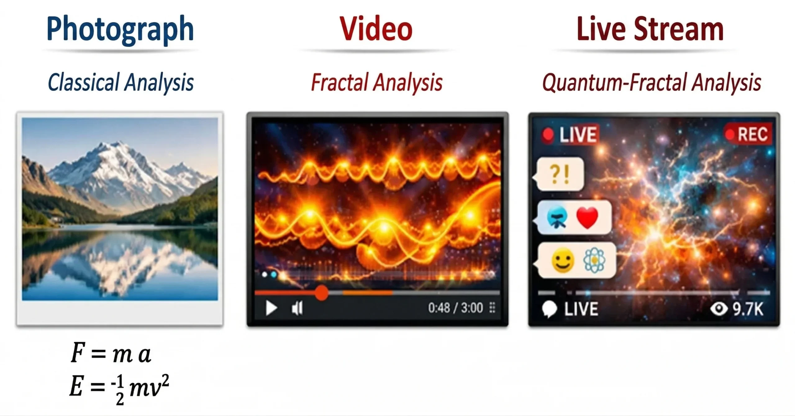
• Photograph (Classical Analysis): A single-frame, stationary image of nature. It represents a “frozen” moment with fixed parameters and linear equations.
• Video (Fractal Analysis): Nature recorded in flow, through processes involving motif-repetition across scales. A dynamic structure where time and resonance are intertwined.
• Live Broadcast (Quantum-Fractal Analysis): Nature as a simultaneous state, constantly reproduced through uncertainty and multiple processes. It means no longer just watching, but flowing together with nature.
  • This topic will be examined in another text.

This trilogy clearly shows the evolution of science: from static to dynamism, from single-scale to multi-scale, from stagnation to resonance.

---

BASIC CONCEPTS

1- Logarithm

Classical Logarithm

Classical definition:

log_b (𝑥) = 𝑦 eger 𝑏^𝑦 = 𝑥

This is a single-scale definition: the base b is constant, and the function operates on a single plane.

Fractal Logarithm

In the fractal version, the base and function become motif-repetitive:

log 𝑏_f (𝑥) = ∑_n=0^∞ 1/𝑏ⁿ ⋅ log 𝑏 (𝑥^{𝑟^n})

Here, r is the fractal scale ratio (e.g., 1/2, 1/3).

Each term represents the repetition of the logarithm at different scales.

Result: Instead of a single value, it produces a fractal spectrum: both micro and macro behaviors are calculated simultaneously.

Properties

• Multi-scale growth: Measures a system’s local and global growth at the same time.
• Motif resonance: Instead of a single logarithmic curve, a chain of motif-repetitive curves emerges.
• New definitions of equilibrium: While the equilibrium point is fixed in classical logarithms, in fractal logarithms, equilibrium is distributed along a motif chain.

Inspiration

Think of it in music: Classical logarithm measures a single pitch. Fractal logarithm measures the resonance of that same sound repeating across octaves. Thus, not only the frequency of a note but its entire fractal harmonic chain is calculated.

GRAPHIC COMPARISON

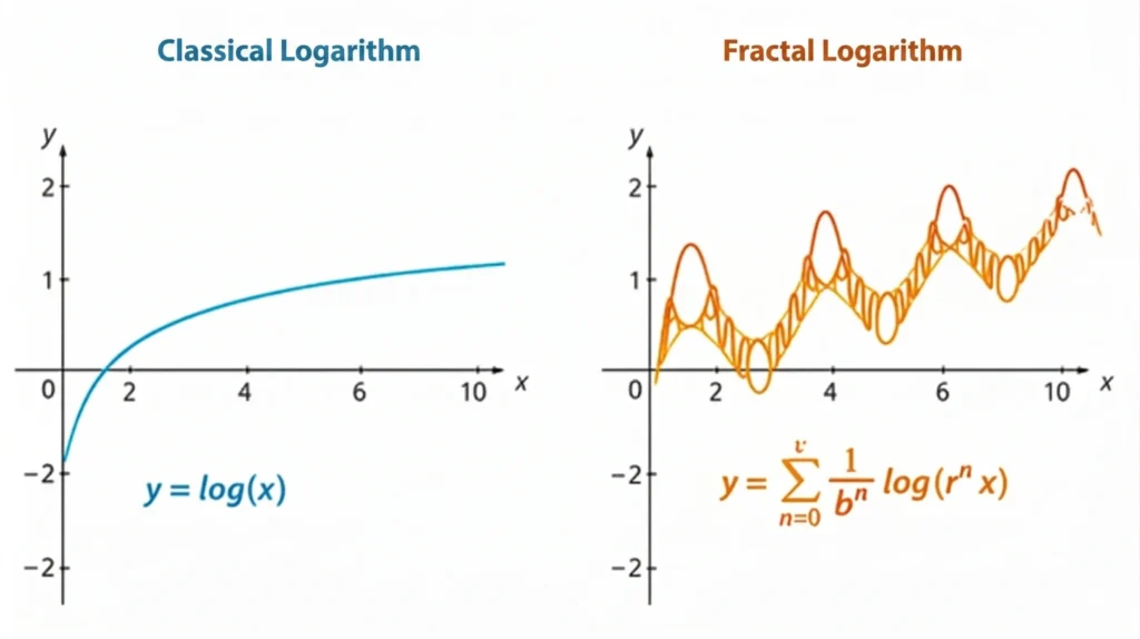
In the visual, you can see the classical logarithm and the fractal logarithm side by side: on the left, the single-scale, smoothly increasing classical curve; on the right, the motif-repetitive, multi-scale fluctuating fractal logarithm.

FORMULA EXPRESSION

1. Basis of Classical Logarithm
   Classical logarithm is the inverse of exponential growth:
   ln (𝑥) = ∫₁^𝑥 (1/𝑡)𝑑𝑡
   This is a single-scale process—the growth rate is constant at every step.
2. The Idea of Fractal Logarithm
   In fractal systems, the growth rate is not constant; every sub-scale has its own rate. Therefore, the logarithm function is expanded as inter-scale integration:
   ln _f (𝑥) = ∫₁^𝑥 (1/𝑡^𝑟(𝑡)) 𝑑𝑡
   Here, r(t) is the fractal ratio function—it determines how “fractal” the system behaves at every point.
3. Discrete Fractal Form
   Instead of continuous integration, the fractal logarithm can be summed across discrete scales:
   ln _f (𝑥) = ∑_k=1^N (1/𝑟^k) ln (𝑥_k)
   Where 𝑥_k is the local growth coefficient of each sub-scale. This expression shows that the classical logarithm becomes a multi-scale sum.
4. Properties
   • If r = 1, it returns to classical ln (𝑥).
   • If r > 1, the logarithm increases more slowly—the fractal density of the system has increased.
   • If r < 1, the logarithm increases faster—the system shows damped fractal behavior.
5. Geometric Meaning
   The fractal logarithm produces a fluctuating function between scales instead of a flat curve. Each sub-scale makes its own logarithmic contribution, explaining the scale-dependent entropy observed in nature.

---

2- EXPONENTIAL FUNCTION

Now let’s derive the definition of the fractal exponential function (𝑒_f^x). This is a motif-repetitive extension of the classical exponential function and the natural complement to the fractal logarithm.

Classical Exponential

Classical definition:

𝑒^x = ∑_n=0^∞ 𝑥^𝑛 / 𝑛!

This is a single-scale series: every term proceeds on the same plane.

Fractal Exponential

In the fractal version, every term becomes scale-repetitive:

𝑒_f^x = ∑_n=0^∞ (𝑥 r^𝑛)^𝑛 / (𝑛! b^𝑛)

• r: fractal scale ratio (e.g., 1/2, 1/3).
• b: motif base, resonance coefficient.Each term represents the repetition of exponential growth at different scales.
  Result: Instead of a single curve, it produces a fractal growth spectrum.

Properties

• Multi-scale growth: Calculates a system’s micro and macro growth simultaneously.
• Motif resonance: Instead of the classical 𝑒^x curve, a chain of motif-repetitive curves emerges.
• New definitions of equilibrium: Growth occurs not just at a single speed, but at different speeds along the motif chain.

Inspiration

Think of it in music: Classical exponential function defines a single crescendo (increase in sound). Fractal exponential function defines the motifs of that same crescendo repeating across octaves. Thus, not just a single rise in a piece, but the entire fractal dynamic chain is calculated.

Application

• Physics: Modeling multi-scale growth processes in chaotic systems.
• Biology: Simultaneously calculating both local and global growth rates in cell division.
• Economics: Defining the fractal growth chains of crisis waves.
• Art/Music: Making motif-repetitive crescendo and rhythm calculations.

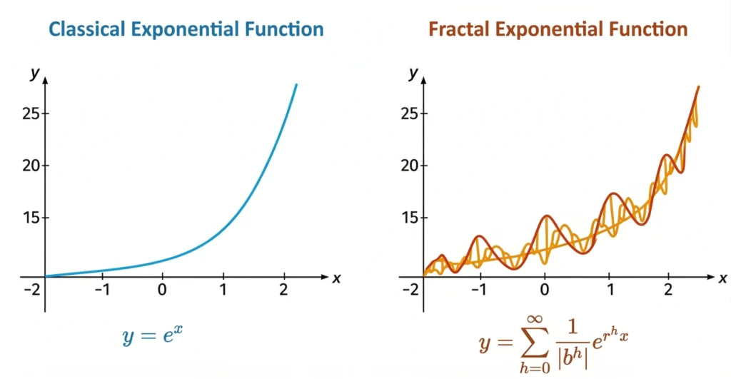
Ready! In this visual, the classical exponential function 𝑦 = 𝑒^x and the fractal exponential function 𝑦 = ∑(1/𝑏ⁿ)𝑒^{r^n x} are shown side by side. While the classical curve on the left displays a smooth, single-scale increase, the fractal curve on the right shows a multi-scale rise with motif-repetitive fluctuations.

This difference visually demonstrates clearly that the fractal exponential carries both micro and macro resonances simultaneously.

Now let’s explain step-by-step how the fractal exponential equation is formed. This is the inverse of the fractal logarithm we just defined—the fundamental function of fractal growth.

1. Classical Exponential Definition
   Classical exponential function:
   𝑒^x = ∑_n=0^∞ 𝑥^𝑛 / 𝑛!
   This is the mathematical expression of single-scale growth—every term increases with the same scale.
2. The Idea of Fractal Exponential
   In fractal systems, every term grows with a different scale. Therefore, every term is scaled with the fractal ratio 𝑟ⁿ:
   𝑒_f^x = ∑_n=0^∞ 𝑥^{𝑛/r^𝑛} / 𝑛!
   Here r is the fractal ratio; it determines the growth coefficient at every sub-scale transition of the system.
3. Alternative Form (Product Form)
   The fractal exponential function can also be written in a multi-scale product form:
   𝑒_f^x = π _k=1^∞ ( 1 + 𝑥/𝑟^k )
   This form is the fractal generalization of the classical 𝑒^x = lim _n→∞ (1 + x/n)ⁿ expression.
4. Properties
   • When r = 1, it returns to classical 𝑒^x.
   • When r > 1, growth is slower but resonant.
   • When r < 1, growth accelerates, and the system shows damped fractal behavior.
   • The fractal exponential function represents the resonance coefficient of continuous growth between scales.
5. Geometric Meaning
   The graph of the fractal exponential function is different from classical 𝑒^x:
   • Instead of a smooth curve, it shows a fluctuating, motif-repetitive rise.
   • Each sub-scale produces its own micro-growth, giving the function a “living” structure.

---

3- Fractal Trigonometric Functions: sin(x) and cos(x)

These are the motif-repetitive, multi-scale extensions of classical sine and cosine.

Classical Definition

They are single-scale wave functions.

Fractal Sine and Cosine

In the fractal version, every term becomes scale-repetitive:

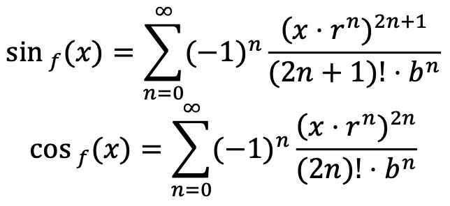
• r: fractal scale ratio (e.g., 1/2, 1/3).
• b: motif base, resonance coefficient.
• Each term represents the repetition of the wave at different scales.
  Result: Instead of a single sine/cosine curve, a fractal wave spectrum is formed.

Properties

• Multi-scale wave: Calculates micro and macro vibrations simultaneously.
• Motif resonance: The wave repeats not just at one frequency, but at different frequencies along the motif chain.
• New definition of period: While the period of classical sine is fixed, the period of fractal sine becomes a motif-repetitive chain.

Inspiration

Think of it in music: Classical sine defines a single pure sound wave. Fractal sine defines the harmonic chain of that same sound repeating across octaves. Thus, not only the fundamental frequency of a note but its entire fractal resonance structure is calculated.

Application

• Physics: Modeling chaotic wave movements (e.g., turbulence, earthquake waves).
• Quantum: Defining new particle interactions with spiral-fractal wave functions.
• Biology: Modeling multi-scale resonances of heart rhythms or brain waves.
• Art/Music: Making fractal harmony and rhythm calculations.

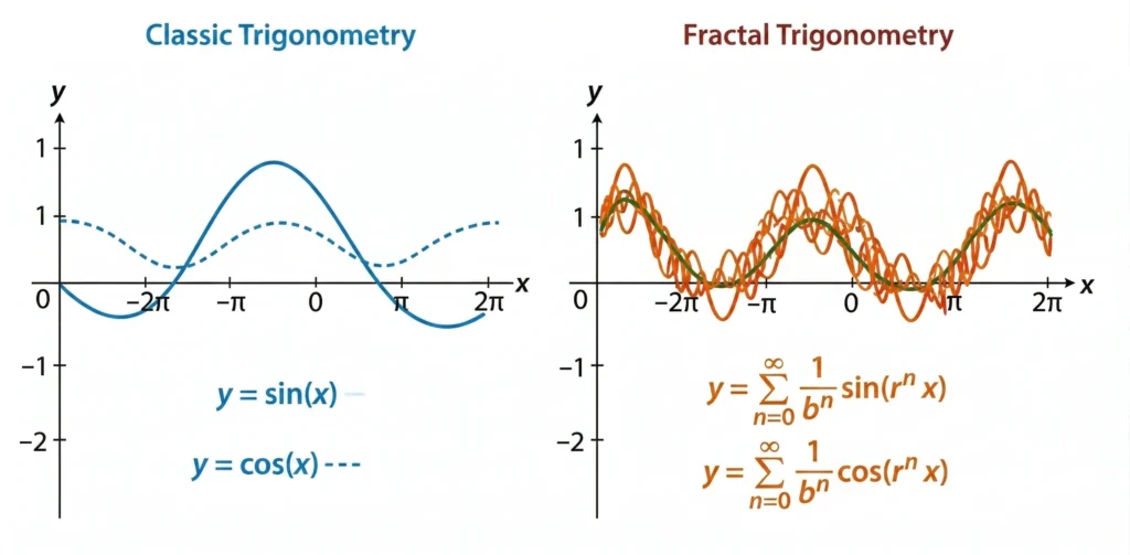
Ready! In this visual, classical trigonometry and fractal trigonometric functions are placed side by side:

On the left, classical 𝑦 = sin (𝑥) and 𝑦 = cos (𝑥) curves form smooth, periodic waves.

On the right, fractal 𝑦 = ∑(1/𝑏ⁿ)sin (𝑟ⁿ𝑥) and 𝑦 = ∑(1/𝑏ⁿ)cos (𝑟ⁿ𝑥) curves display motif-repetitive, multi-scale fluctuations.

This difference visually demonstrates clearly that fractal trigonometric functions have a much more complex and multi-scale structure than classical waves.

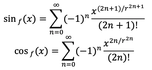
Let’s explain step-by-step how fractal trigonometric functions are formed. This is the expansion of classical sine and cosine functions via fractal calculus.

1. Classical Definition
   Classical trigonometric functions are derived from exponential functions:
   sin (𝑥) = ( 𝑒^𝑖𝑥 − 𝑒^-𝑖𝑥 ) / 2𝑖 , cos (𝑥) = ( 𝑒^𝑖𝑥 + 𝑒^-𝑖𝑥 ) / 2
2. Fractal Exponential Base
   The basis of fractal trigonometric functions is the fractal exponential function:
   𝑒_f ^𝑖𝑥 = π_k=1^∞ ( 1 + 𝑖𝑥/𝑟^k )
   Here r is the fractal ratio, determining the growth coefficient for each sub-scale.
3. Definition of Fractal Sine and Cosine
   Using the fractal exponential function:
   sin_f (𝑥) = ( 𝑒_f ^𝑖𝑥 − 𝑒_f ^-𝑖𝑥 ) / 2𝑖
   cos_f (𝑥) = ( 𝑒_f ^𝑖𝑥 + 𝑒_f ^-𝑖𝑥 ) / 2
4. Discrete Series Form
   Fractal trigonometric functions are the fractal generalization of the classical Taylor series:

5. Properties

• When r = 1, classical sin (𝑥) and cos (𝑥) are obtained.
• When r > 1, the functions become more “wavy” and resonant.
• When r < 1, the functions oscillate faster, showing damped fractal behavior.

6. Geometric Meaning
Fractal trigonometric functions produce multi-scale wave networks instead of classical smooth waves. Each sub-scale makes its own sine/cosine contribution, resulting in motif-repetitive, resonant waves.

---

4- Let’s move to the Fractal Fourier Transform (FFT), the natural continuation of fractal trigonometric functions.

This is a multi-scale, motif-repetitive expansion of the classical Fourier transform and takes wave decomposition to a brand new dimension.

Classical Fourier Transform

𝐹(𝜔) = ∫_-∞^∞ 𝑓(𝑥) 𝑒^-i𝜔𝑥 𝑑𝑥

This definition decomposes a function on a single frequency axis.

Fractal Fourier Transform

In the fractal version, the integral becomes scale-repetitive:

𝐹_f (𝜔) = ∑_n=0^∞ (1/𝑏ⁿ) ∫_-∞^∞ 𝑓(𝑟ⁿ𝑥) 𝑒^{-i𝜔(r^n)𝑥} 𝑑𝑥

• r: fractal scale ratio (e.g., 1/2, 1/3).
• b: motif base, resonance coefficient.Each term represents the Fourier decomposition of the function at different scales.
  Result: Instead of a single frequency spectrum, a fractal frequency spectrum is formed.

Properties

• Multi-scale frequency decomposition: Extracts both micro and macro frequency components simultaneously.
• Motif resonance: Frequency repeats not just on one axis, but along the motif chain.
• New spectrum definition: While there is a single spectrum in classical Fourier, in fractal Fourier, the spectrum is distributed along a motif chain.

Inspiration

Think of it in music: Classical Fourier decomposes a melody into its fundamental frequencies. Fractal Fourier decomposes the same melody into a motif chain repeating across octaves. Thus, not only the fundamental frequencies but the entire fractal harmony structure is revealed.

Application

• Physics: Multi-scale frequency analysis of turbulence, earthquake waves, and chaotic flows.
• Quantum: Decomposition of spiral-fractal wave functions.
• Biology: Fractal frequency spectra of brain waves and heart rhythms.
• Data Analysis: Motif-repetitive decomposition of crisis waves in financial time series.
• Art/Music: Analysis of fractal harmony and rhythm compositions.

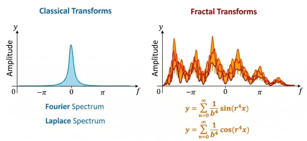
Ready! In this visual, the single-peak spectra of classical Fourier and Laplace transforms are side by side with the motif-repetitive, multi-scale spectra of fractal Fourier and Laplace transforms. While the classical spectra on the left have a sharp, single-frequency peak, the fractal spectra on the right form a wide, layered frequency range.

This difference visually shows clearly that fractal transforms reveal much richer and multi-scale frequency components in signal analysis.

Let’s explain step-by-step how fractal Fourier and fractal Laplace transforms are formed. This is the expansion of classical transforms via fractal calculus.

1. Classical Fourier Transform
   Classical definition:
   𝐹(𝜔) = ∫_-∞^∞ 𝑓(𝑡) 𝑒^-i𝜔𝑡 𝑑𝑡
   This is the representation of the function in frequency space.
2. Fractal Fourier Transform
   In fractal systems, every frequency component resonates at different scales. Therefore:
   𝐹_f (𝜔) = ∫_-∞^∞ 𝑓(𝑡) 𝑒_f^-i𝜔𝑡 𝑑𝑡
   Here 𝑒_f^-i𝜔𝑡 is the fractal exponential function.
   Discrete form:
   𝐹_f (𝜔) = ∑_k=1^∞ ∫ 𝑓(𝑡) 𝑒^{-i𝜔𝑡 / r^k} 𝑑𝑡
   Each sub-scale (𝑟^k) makes its own frequency contribution. Thus, a fractal spectrum network is obtained instead of a classical Fourier spectrum.
3. Classical Laplace Transform
   Classical definition:
   𝐿(𝑠) = ∫₀^∞ 𝑓(𝑡) 𝑒^-s 𝑑𝑡
   This is the transform of the function from time space to the complex plane.
4. Fractal Laplace Transform
   In fractal systems, the damping coefficient is not single-scale, but multi-scale:
   𝐿_f (𝑠) = ∫₀^∞ 𝑓(𝑡) 𝑒_f^-s𝑡 𝑑𝑡
   Discrete form:
   𝐿_f (𝑠) = ∑_k=1^∞ ∫ 𝑓(𝑡) 𝑒^{-s𝑡 / r^k} / 𝑑𝑡
   Each sub-scale produces a different damping coefficient. This reveals the multi-scale time resolution of the system.
5. Properties
   • When r = 1, it returns to classical Fourier and Laplace transforms.
   • When r > 1, the spectrum becomes wider and more resonant.
   • When r < 1, the spectrum becomes narrower and damped.
   • Fractal transforms are the inter-scale generalization of classical transforms.
6. Geometric Meaning
   • Fractal Fourier: Multi-scale frequency network instead of a single frequency → modeling complex vibrations in nature.
   • Fractal Laplace: Multi-scale damping instead of single damping → modeling complex time flows in nature.

---

5- Let’s complete with fractal differential equations (𝐷_f).

This is a motif-repetitive, multi-scale expansion of classical differential equations and opens brand new horizons in analyzing the dynamics of systems.

Classical Differential Equation

Example:

𝑑𝑦 / 𝑑𝑡 = 𝑓(𝑡, 𝑦)

This is a single-scale definition: change is calculated in only one time scale.

Fractal Differential Equation

In the fractal version, the derivative becomes scale-repetitive:

𝐷_f 𝑦(𝑡) = ∑_n=0^∞ (1/𝑏ⁿ)(𝑑𝑦/𝑑𝑡)(rⁿ𝑡)

• r: fractal scale ratio (e.g., 1/2, 1/3).
• b: motif base, resonance coefficient.
• Each term represents the derivative of the system at different scales.
  Result: Instead of a single derivative, a fractal derivative chain is formed.

Properties

• Multi-scale dynamics: Solves micro and macro changes simultaneously.
• Motif resonance: The system response is not just a single derivative, but derivatives repeating along the motif chain.
• New solution space: Instead of classical solutions, fractal solutions—that is, motif-repetitive function families—emerge.

Inspiration

Think of it in music: Classical differential equation defines the change of a melody at a single speed. Fractal differential equation defines the speed changes of the same melody repeating across octaves. Thus, not just a single tempo, but the entire fractal tempo chain is calculated.

Application

• Physics: Multi-scale dynamic solution of chaotic flows and earthquake waves.
• Quantum: Differential solution of spiral-fractal wave functions.
• Biology: Fractal dynamics of cell division, signaling pathways, and protein folding.
• Economics: Motif-repetitive differential models of crisis waves.
• Art/Music: Fractal tempo and dynamic calculations.

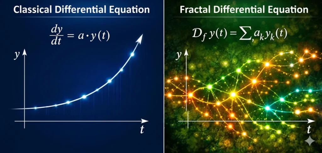
Ready! Here is the visualization showing classical and fractal differential equations side by side:

• Classical Differential Equation: 𝑑𝑦/𝑑𝑡 = 𝑎 ⋅ 𝑦(𝑡). A single-scale, smooth curve. A function that grows or decays continuously and at a constant rate over time.
• Fractal Differential Equation: 𝐷_f 𝑦(𝑡) = ∑𝑎_k 𝑦_k (𝑡). A multi-scale, branching structure. Each sub-scale makes its own contribution, resulting in a resonant and motif-repetitive network.

This comparison clearly shows that classical differential equations display nature in a single line like a “photograph”; fractal differential equations reveal nature as a multi-scale, branching “video”.

1. Basis of Classical Differential Equation
   Classical form:
   𝑑𝑦/𝑑𝑡 = 𝑎 ⋅ 𝑦(𝑡)
   Where 𝑎 is a constant rate and 𝑦(𝑡) is a function that changes over time. This equation expresses a single-scale, smooth growth or decay process.
2. Concept of Fractal Derivative
   In fractal systems, the rate of change is not constant; every sub-scale has its own speed. Therefore, a fractal derivative operator is defined instead of the classical derivative:
   𝐷_f 𝑦(𝑡) = (𝑑^r(𝑡)𝑦) / (𝑑𝑡^r(𝑡))
   Where 𝑟(𝑡) is the fractal ratio function—it determines how fractal the system behaves at every point.
3. Definition of Fractal Differential Equation
   If the classical equation is expanded with the fractal derivative:
   𝐷_f 𝑦(𝑡) = 𝑎_f (𝑡) ⋅ 𝑦(𝑡)
   Here 𝑎_f (𝑡) is no longer a constant, but an inter-scale resonance coefficient. This shows that the system changes at different speeds at every sub-scale transition.
4. Discrete Fractal Form
   A fractal differential equation can be written as a sum of sub-scales:
   𝐷_f 𝑦(𝑡) = ∑_k=1^N 𝑎_k 𝑦_k (𝑡)
   Each 𝑦_k (𝑡) is a sub-scale function; each has its own resonance coefficient 𝑎_k. This form mathematically captures the multi-scale interaction in nature.
5. Solution Form
   The solution to the fractal differential equation is expressed with a fractal exponential function instead of a classical exponential:
   𝑦(𝑡) = 𝑦₀ ⋅ 𝑒_f ^{∫ 𝑎_f (𝑡)𝑑𝑡}
   This expresses that the system shows a fluctuating, motif-repetitive growth over time.
6. Geometric and Physical Meaning
   • Classical: Single line, constant speed, stationary process.
   • Fractal: Branching, resonance, interaction between scales. Each sub-scale produces its own micro-dynamics; the total behavior of the system is the combination of these micro-fluctuations.

---

6- Fractal Integral (∫_f)

This makes the classical integral motif-repetitive and opens brand new horizons, especially in calculations like energy, field, and probability.

Classical Integral

𝐼 = ∫ 𝑓(𝑥) 𝑑𝑥

It is a single-scale summation: it calculates the area of the function on a single plane.

Fractal Integral

In the fractal version, the integral becomes scale-repetitive:

∫_f 𝑓(𝑥) 𝑑𝑥 = ∑_n=0^∞ (1/𝑏ⁿ) ∫ 𝑓(𝑟ⁿ𝑥) 𝑑𝑥

• r: fractal scale ratio (e.g., 1/2, 1/3).
• b: motif base, resonance coefficient.
• Each term represents the integral of the function at different scales.
  Result: Instead of a single area, a fractal area spectrum is formed.

Properties

• Multi-scale total: Sums micro and macro contributions simultaneously.
• Motif resonance: The area repeats not just on one plane, but along the motif chain.
• New definition of probability: While probability is a single distribution in classical integrals, in fractal integrals, the distribution becomes a motif-repetitive chain.

Inspiration

Think of it in music: Classical integral measures the total sound energy of a piece. Fractal integral measures the energy chain of that same piece repeating across octaves. Thus, not just a single total, but the entire fractal energy structure is calculated.

Application

• Physics: Multi-scale calculation of energy densities (e.g., earthquake energy, cosmic flows).
• Quantum: Field integrals of spiral-fractal wave functions.
• Biology: Motif-repetitive calculation of intracellular energy distribution.
• Economics: Fractal integral of the total impact of crisis waves.
• Art/Music: Total resonance energy of fractal motifs.

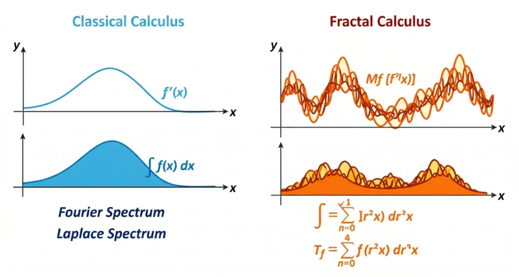
Ready! In this visual, classical derivative/integral curves and fractal derivative/integral chains are side by side:

• On the left, classical derivative 𝑓 ‘ (𝑥) and integral ∫ 𝑓(𝑥)𝑑𝑥 draw smooth, single-scale curves.
• On the right, fractal derivative 𝑀_f [𝑓 ‘ (𝑥)] and fractal integral 𝑇_f ∫ 𝑓(𝑟ⁿ𝑥)𝑑𝑟ⁿ𝑥 form motif-repetitive, multi-scale curves.

This difference visually demonstrates clearly that fractal calculus can perform a much more complex, multi-scale analysis than classical derivative and integral.

Let’s explain step-by-step the formation of fractal derivative and fractal integral equations. These two concepts transform classical calculus’s understanding of “single-scale change” into a multi-scale, resonant structure.

1. Basis of Classical Derivative and Integral
   Classical derivative:
   𝑑𝑦/𝑑𝑥 = lim _Δ𝑥→0 (𝑦(𝑥 + Δ𝑥) − 𝑦(𝑥)) / Δ𝑥
   Classical integral:
   ∫ 𝑦(𝑥) 𝑑𝑥 = lim_Δ𝑥→0 ∑𝑦(𝑥) Δ𝑥
   Both operations measure single-scale change—that is, they examine nature with a flat, fixed lens.
2. The Idea of Fractal Derivative
   In fractal systems, the rate of change is different for every scale. Therefore, the derivative is defined as an inter-scale sum:
   𝐷_f 𝑦(𝑥) = ∑_k=1^N (𝑦(𝑥 + Δ𝑥_k) − 𝑦(𝑥)) / Δ𝑥_k^r_k
3. The Idea of Fractal Integral
   The fractal integral is the inter-scale generalization of the classical sum:
   𝐼_f = ∑_k=1^N 𝑦(𝑥_k) Δ𝑥_k^r_k
   Each sub-scale contributes its own “micro-area.” This represents the multi-scale accumulation in nature—flow of energy, information, or matter.
4. Continuous Fractal Form
   If we write it in continuous form:
   𝐷_f 𝑦(𝑥) = ∫₀^∞ ( ∂𝑦(𝑥, 𝑟) / ∂𝑥 ) 𝑑𝑟
   𝐼_f = ∫₀^∞ 𝑦(𝑥, 𝑟) 𝑑𝑟
   Here r is no longer a parameter, but a scale space—it represents the resonance dimension of the system.
5. Properties
   • When r = 1, classical derivative and integral are obtained.
   • r > 1: the system shows slower, resonant change.
   • r < 1: the system shows faster, damped change.
   • Fractal derivative and integral mathematically express the continuity between scales in nature.
6. Geometric Meaning
   • Classical derivative: Single line, constant slope.
   • Fractal derivative: Branching, micro-fluctuation, resonant slope.
   • Classical integral: Smooth area.
   • Fractal integral: Motif-repetitive, multi-scale area accumulation.